
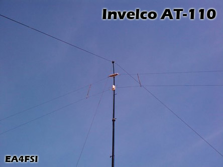
Invelco AT-110 folded dipole antenna
|
Main → HF Radio Resources Center → HF Antennas → Invelco AT-110 → Simulation (model 1) |
![]() Este artículo también está disponible en Español (this article is also available in Spanish).
Este artículo también está disponible en Español (this article is also available in Spanish).
5. Simulation of the AT-110A antenna (model 1).
In this section I will show the results of the simulations performed with the Invelco AT-110A antenna 4Nec2 model 1, presented in the section 2. The values of L, S, R and Phi can be consulted in the antenna's user manual.
In all the simulations, a ground of average type is considered, with a conductivity of 0.005 S/m and a dielectric constant of 13.
I have used discrete frequencies in all the working range of the antenna (2-30 MHz), at 1 MHz intervals or even at 200 kHz intervals when necessary.
On the other hand, the SWR calculations will be referred to a characteristic impedance of 450 ohms (9:1 balun in order to work with 50 ohms radios).
I have simulated configurations with masts of lengths HM equal to 9 m, 12 m, 15 m and 18 m, being for all of them the height of installation of the tips HE equal to 0,5 m. In those four cases, the angle between the two legs of the antena will be of 144º, 131º, 117º and 102º, respectively.
Finally, in all the simulations a resolution of 1 degree will be used.
5.1. Computation of the standing wave ratio (SWR).
The fig.5 shows the SWR vs frequency plots resulting from the simulations of the model 1. Click on the image to see a larger version.
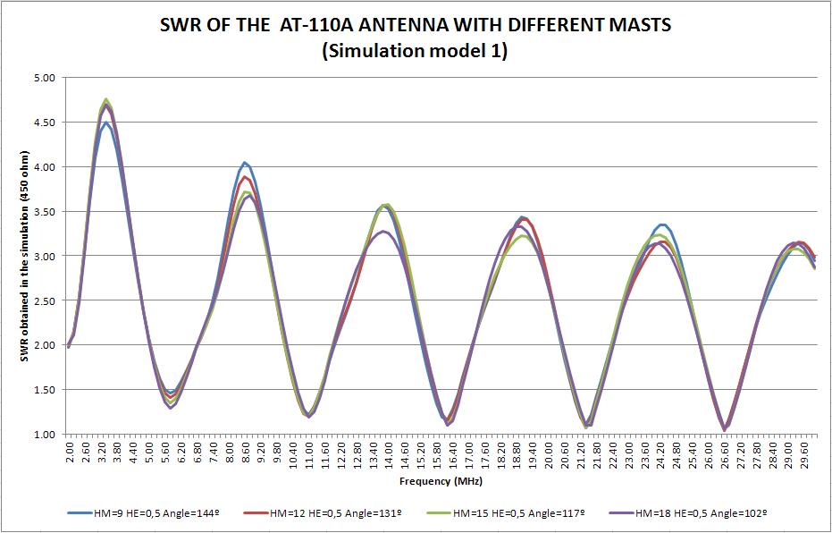
The results will be analysed in the section 7.
5.2. Simulation of radiation patterns.
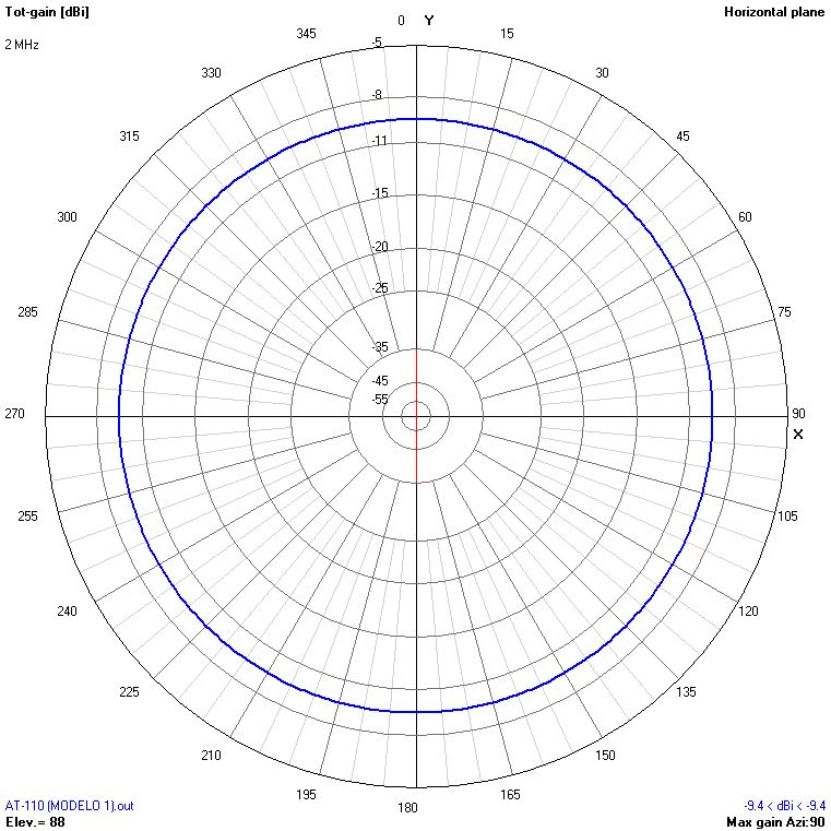
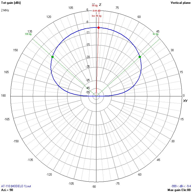
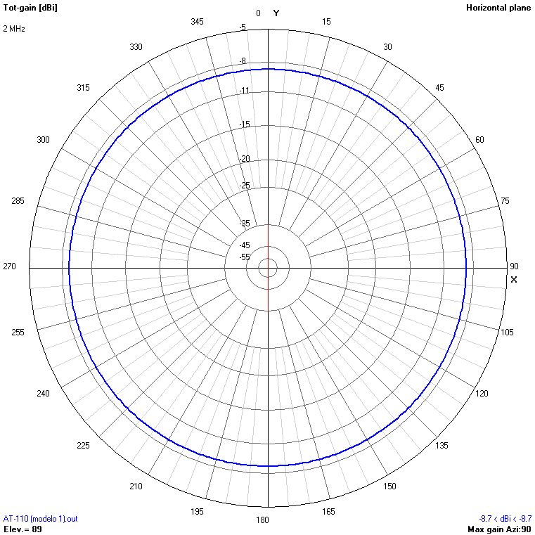
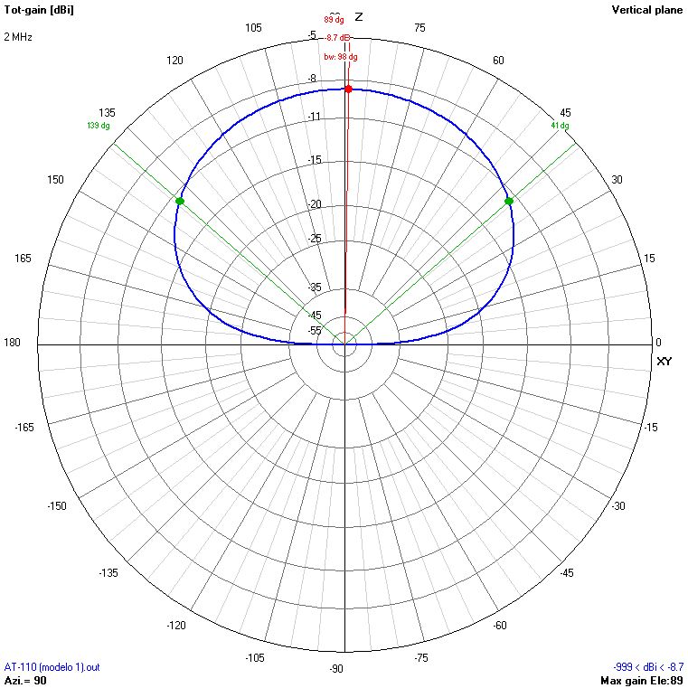
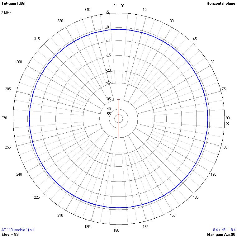
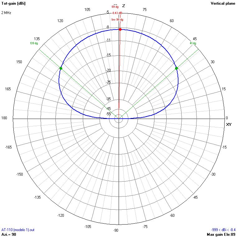
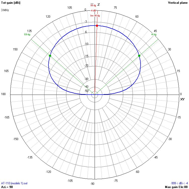
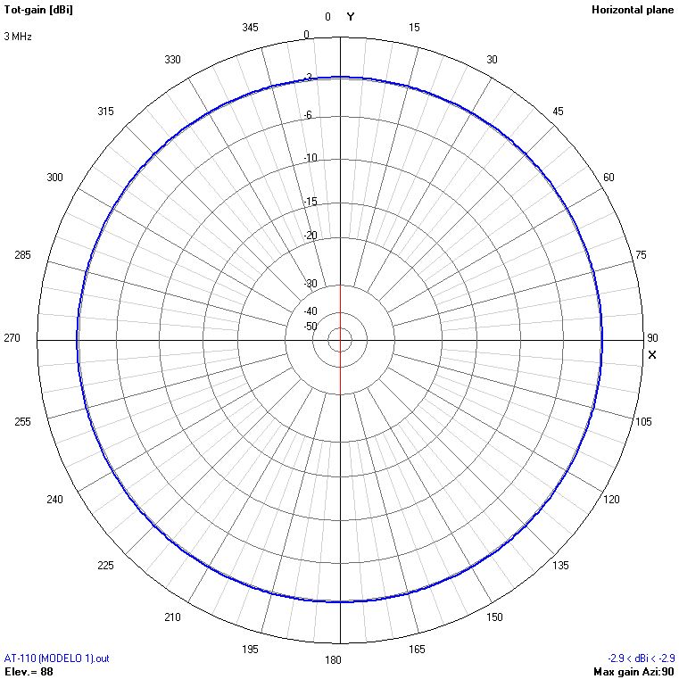
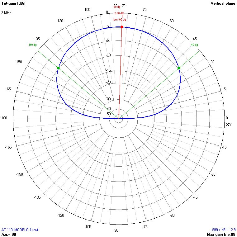
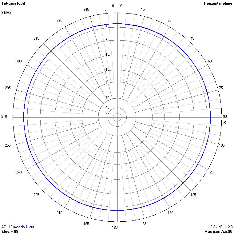
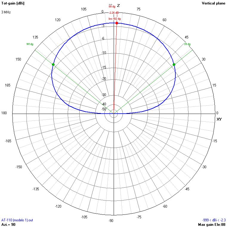
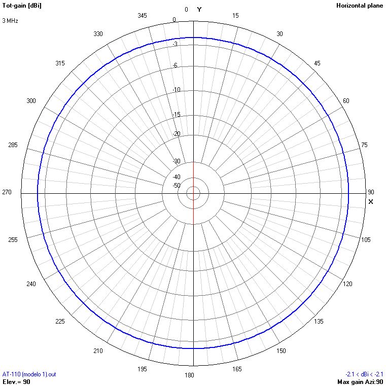
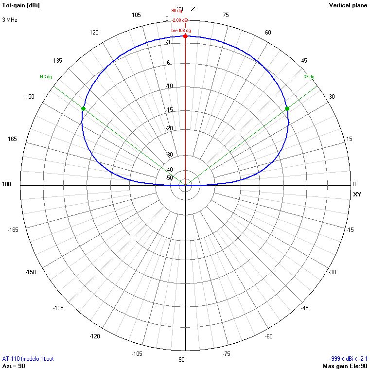
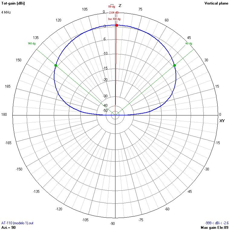
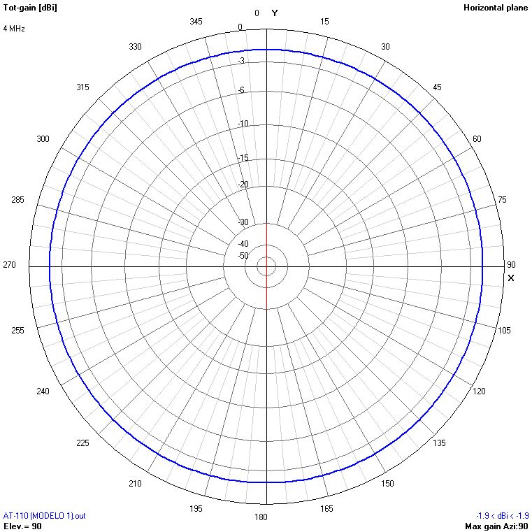
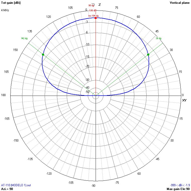
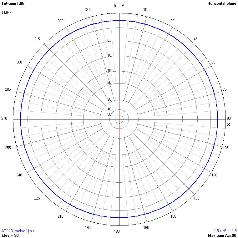
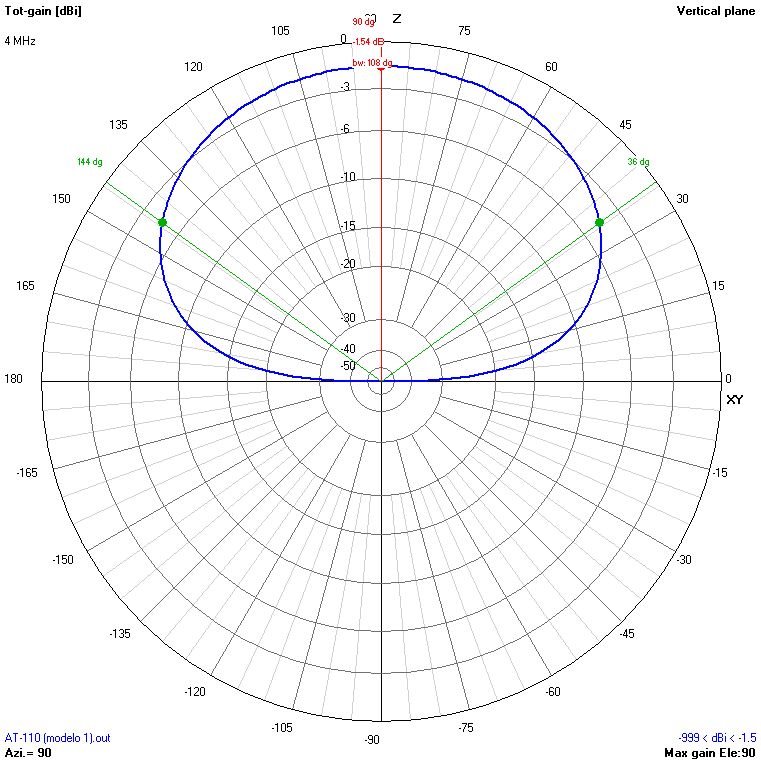
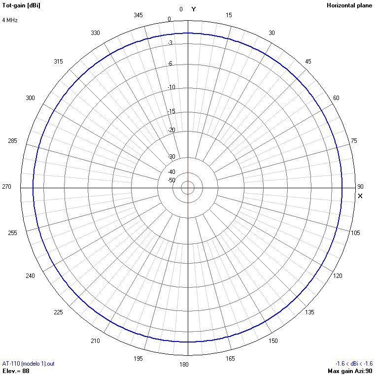
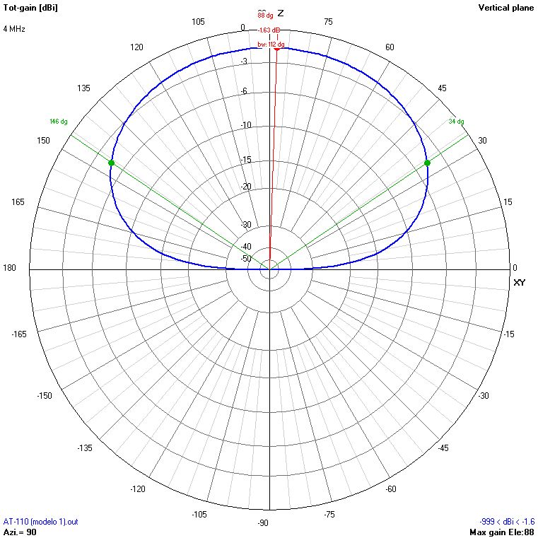
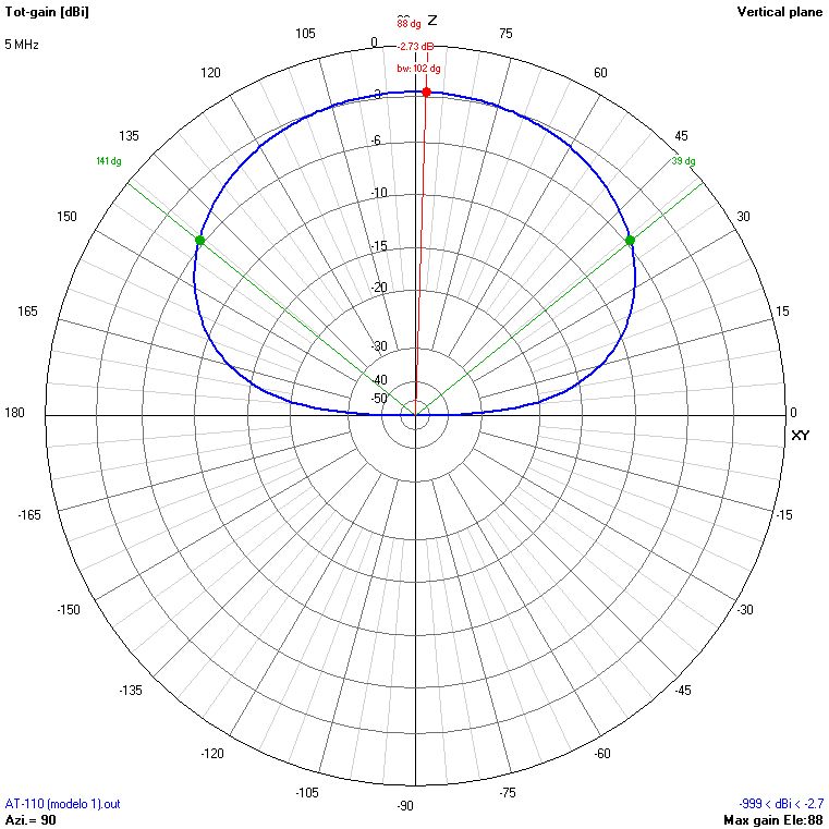
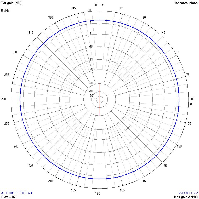
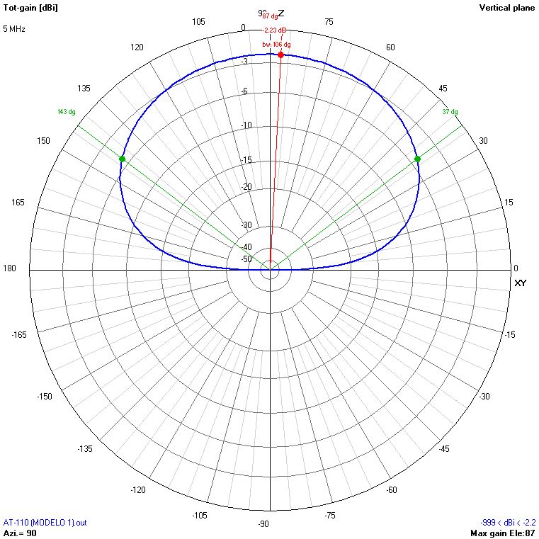
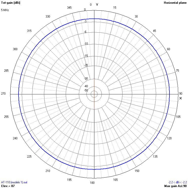
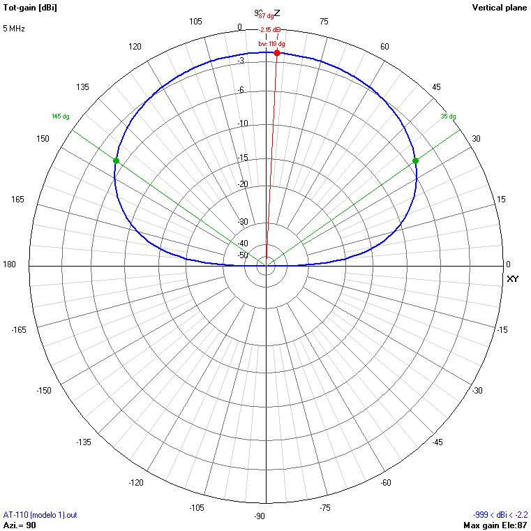
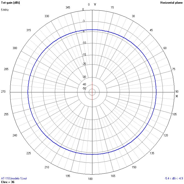
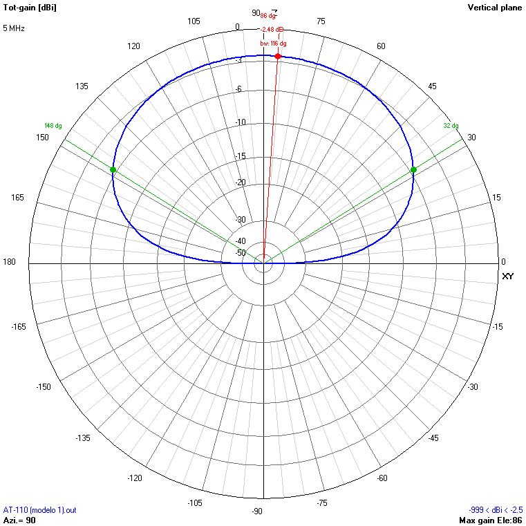
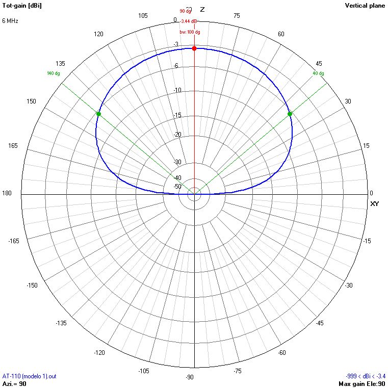
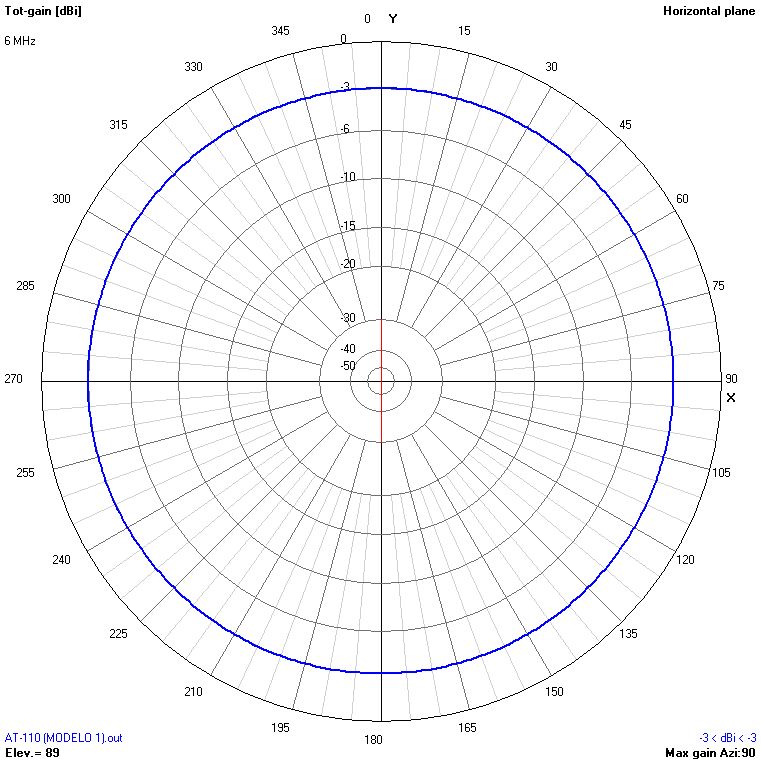
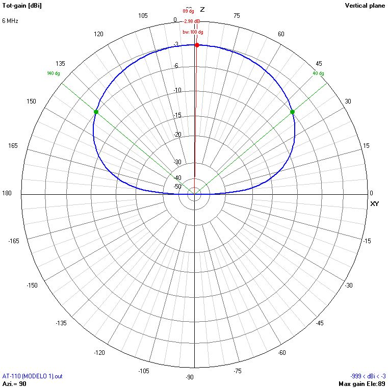
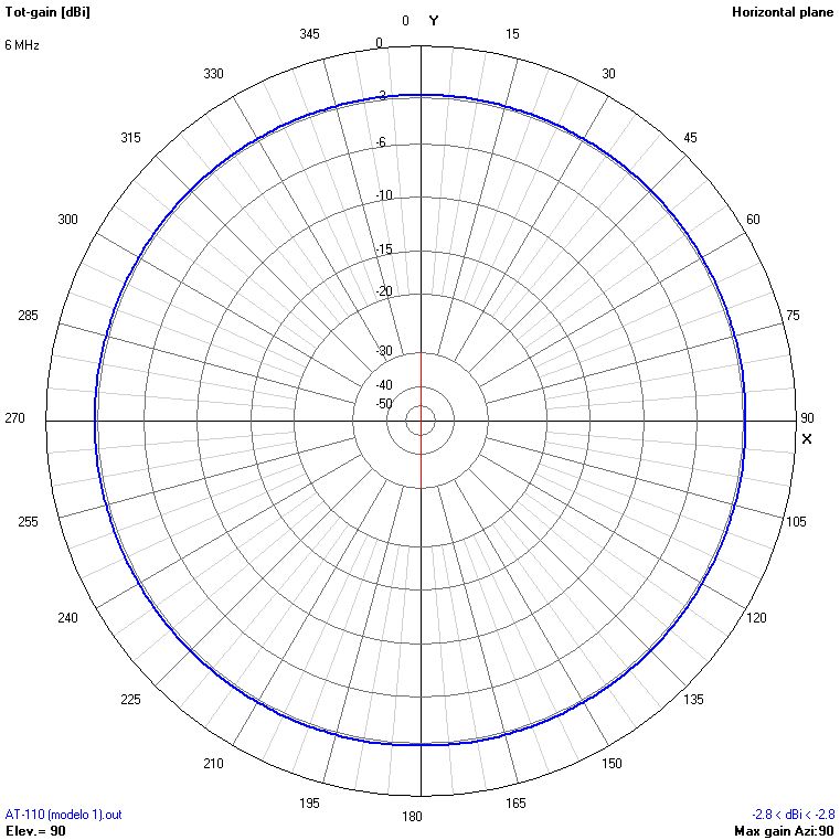
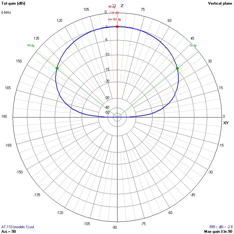
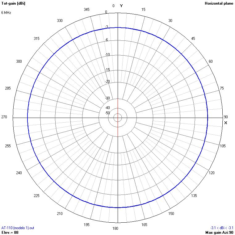
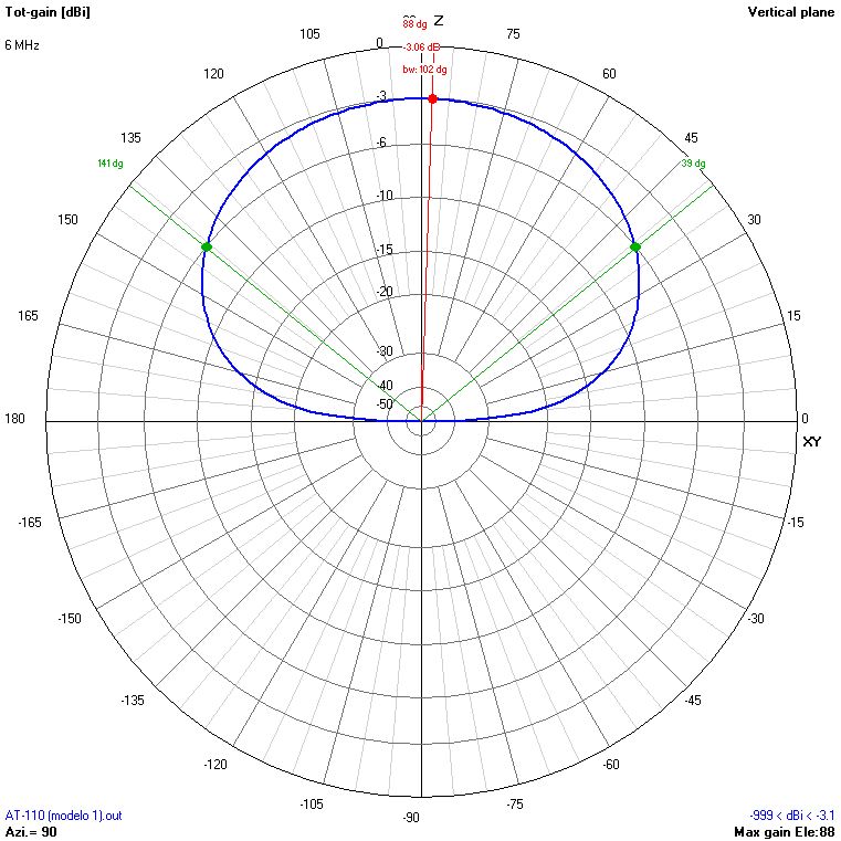
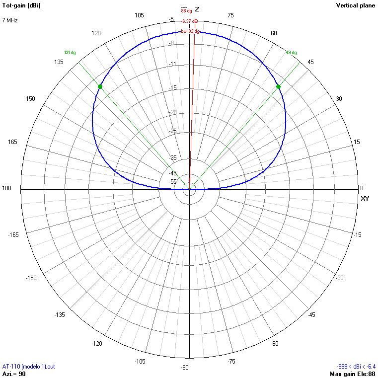
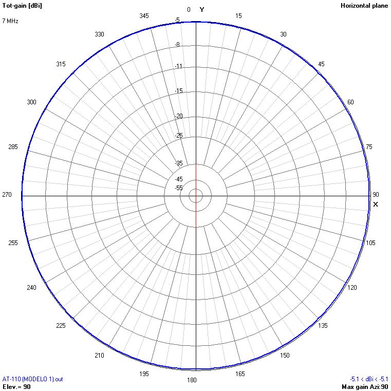
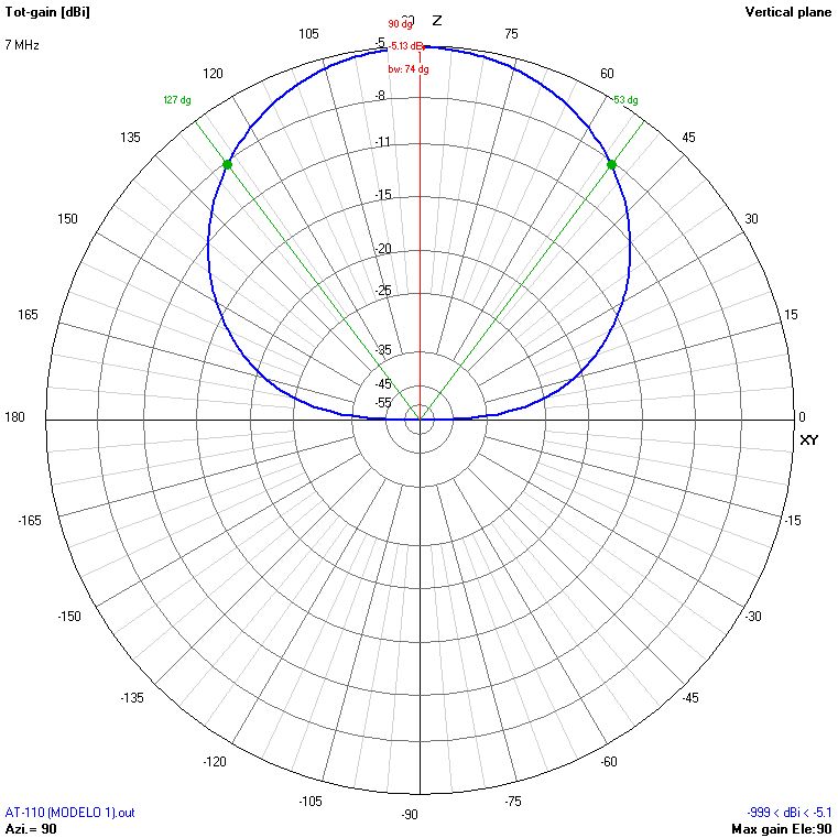
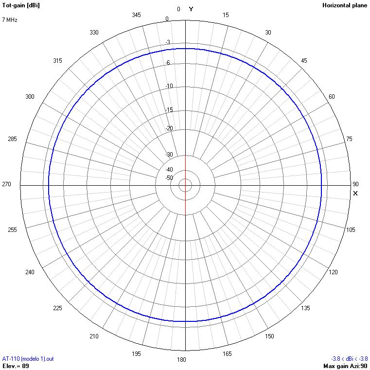
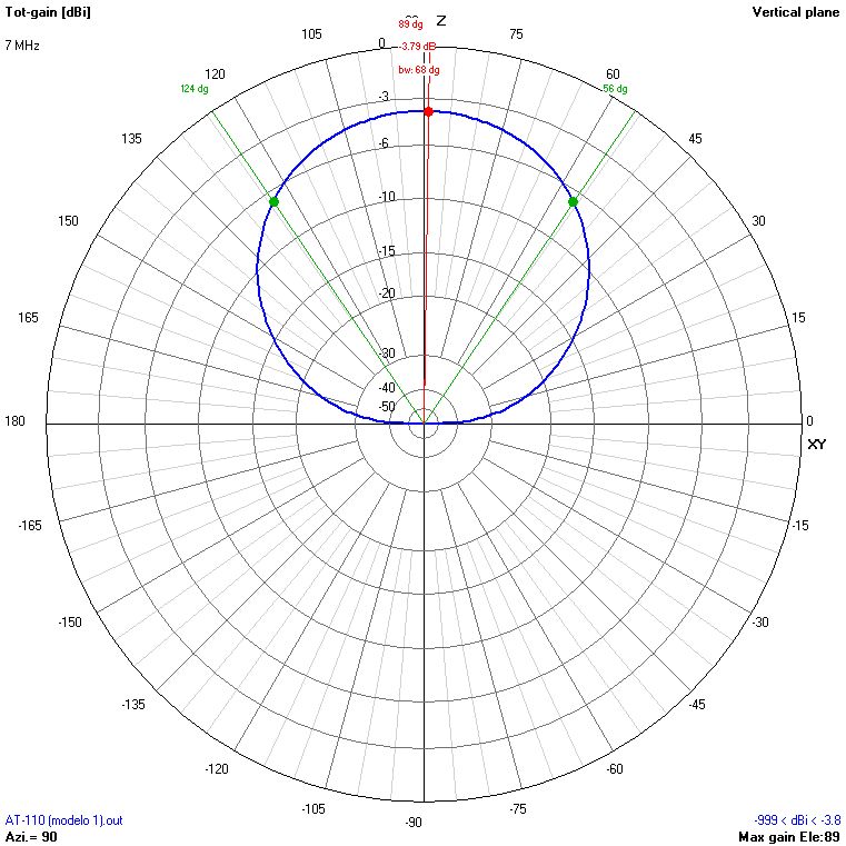
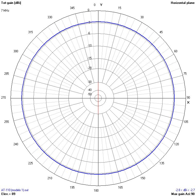
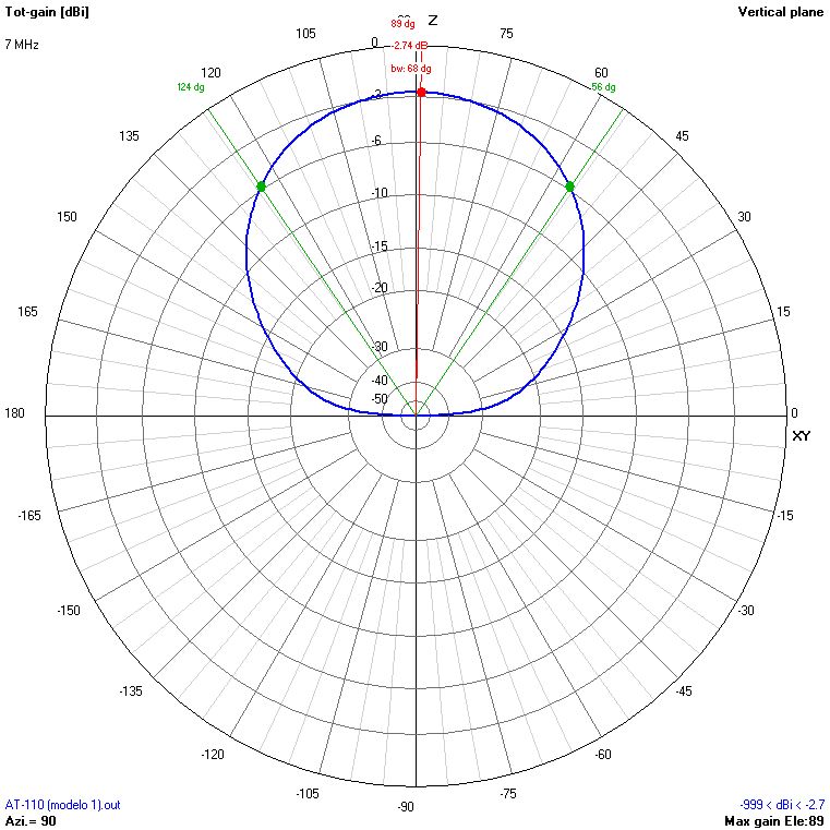
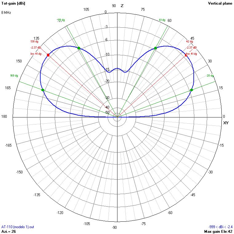
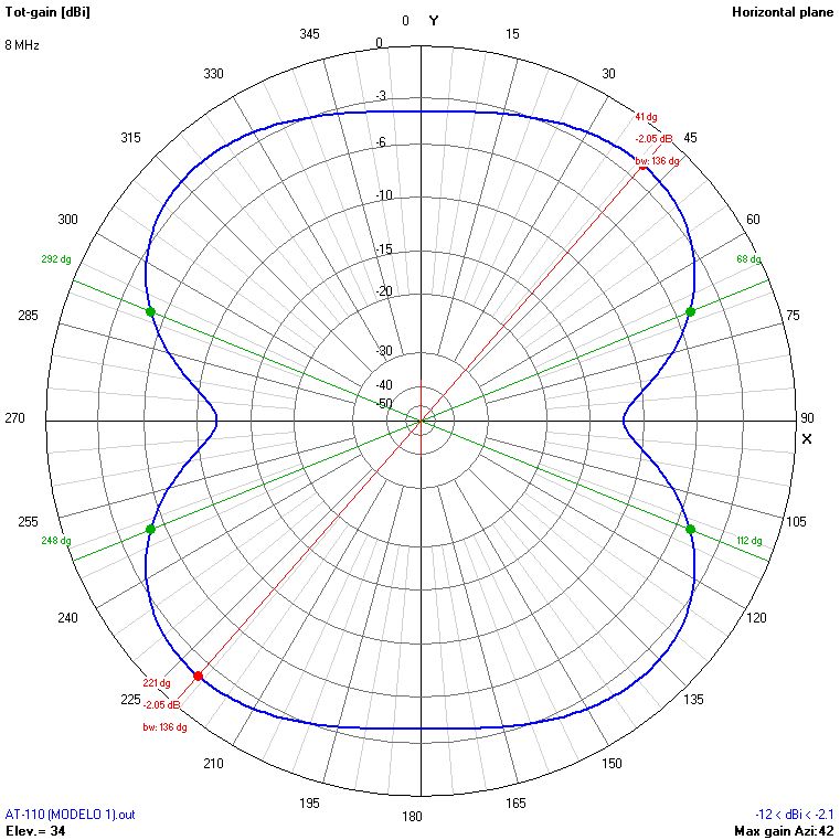
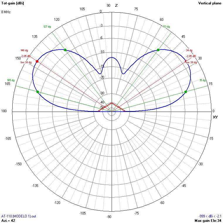
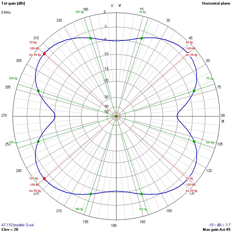
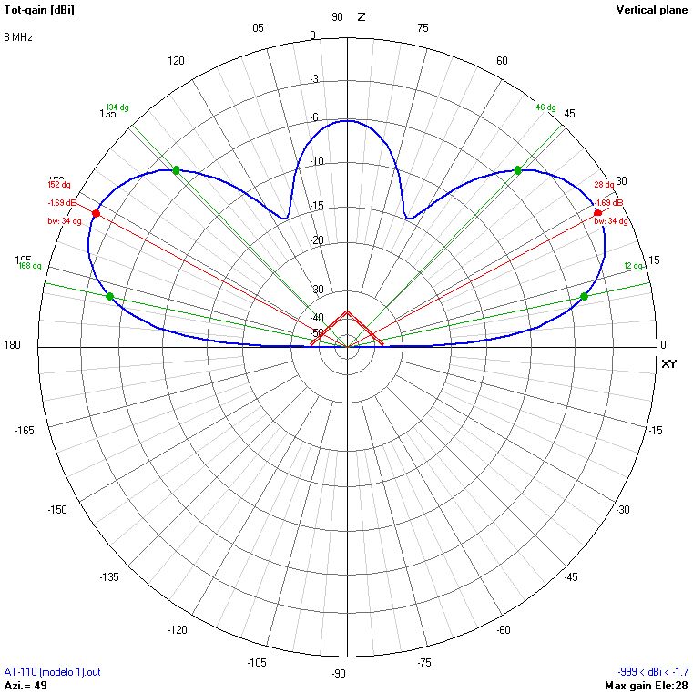
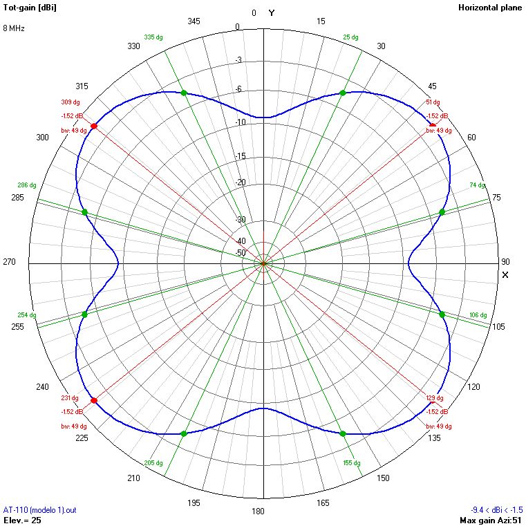
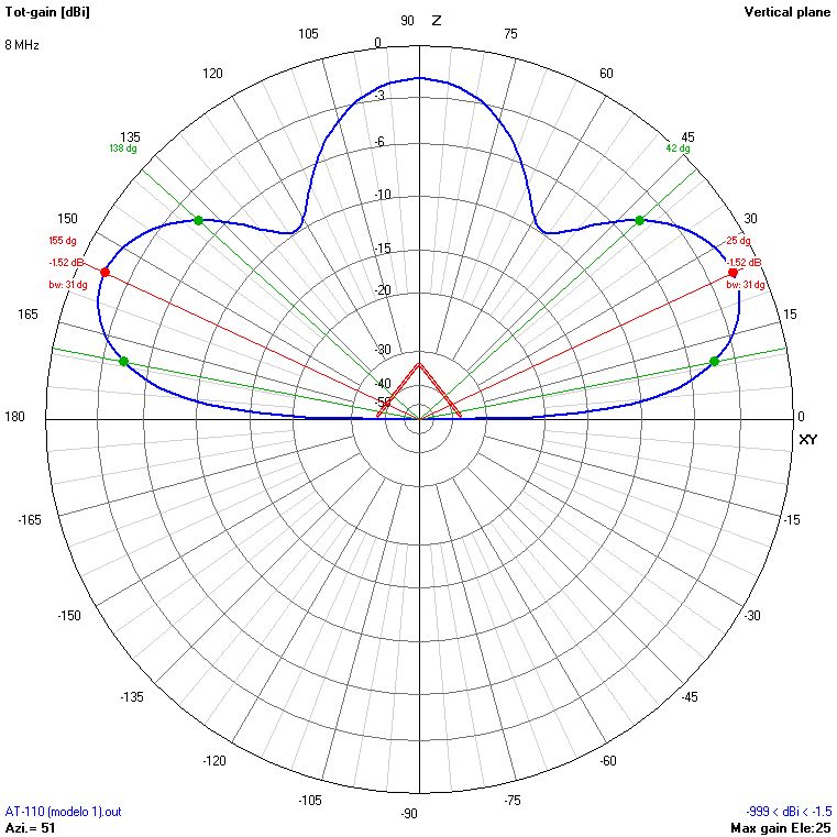
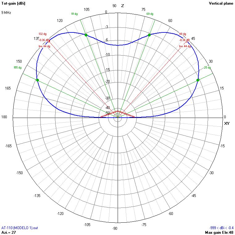
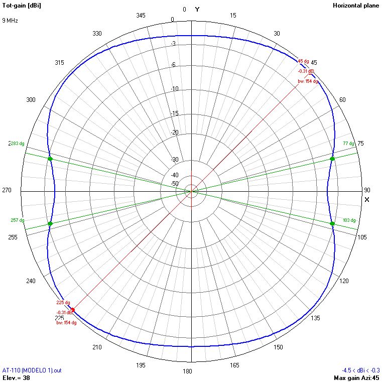
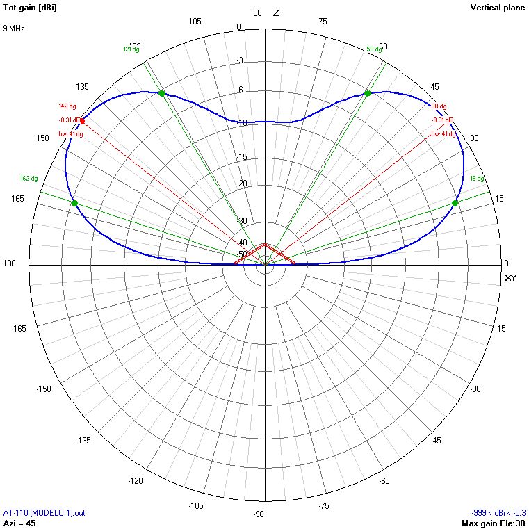
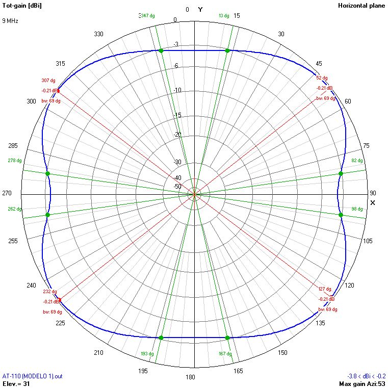
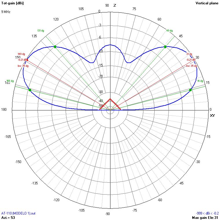
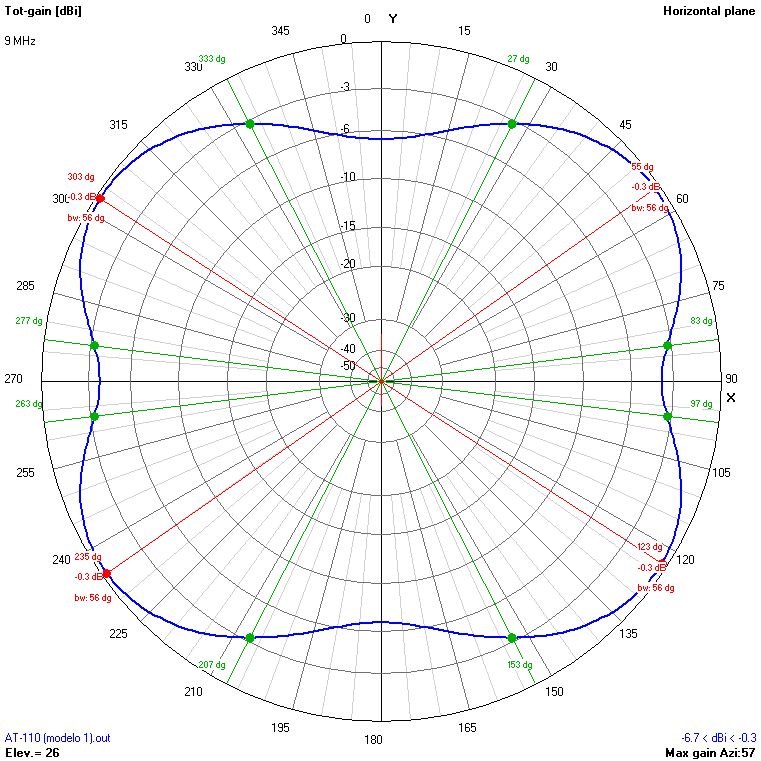
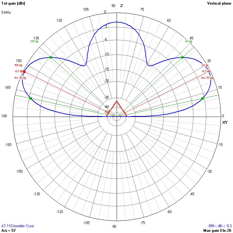
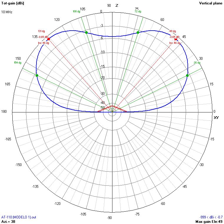
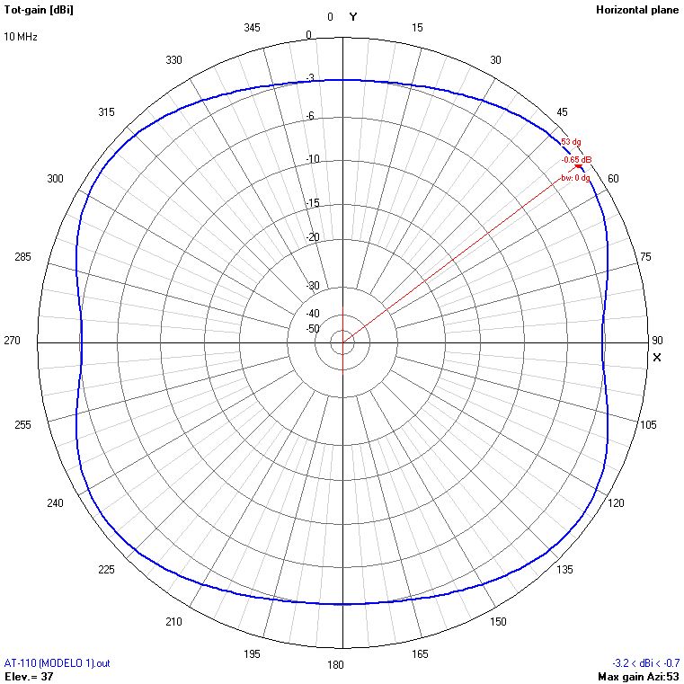
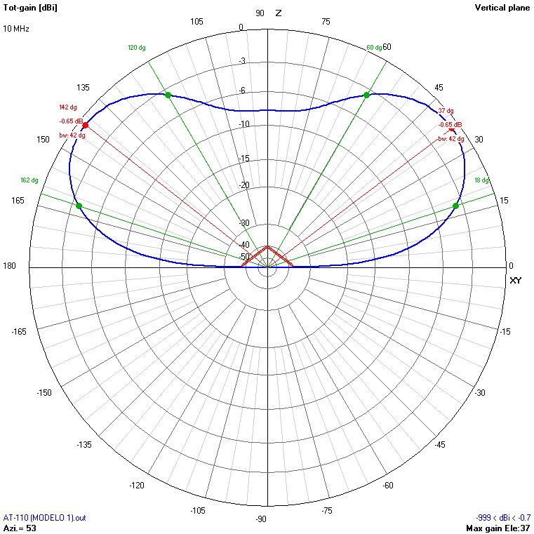
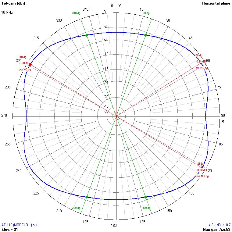
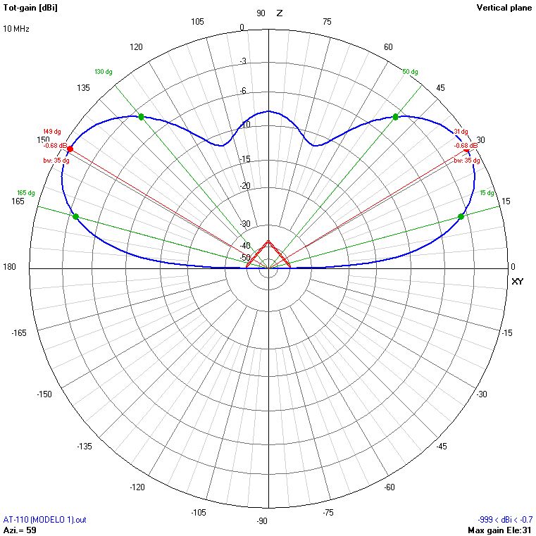
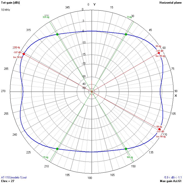
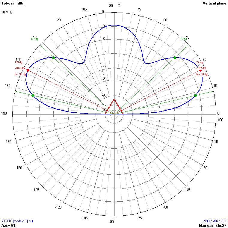
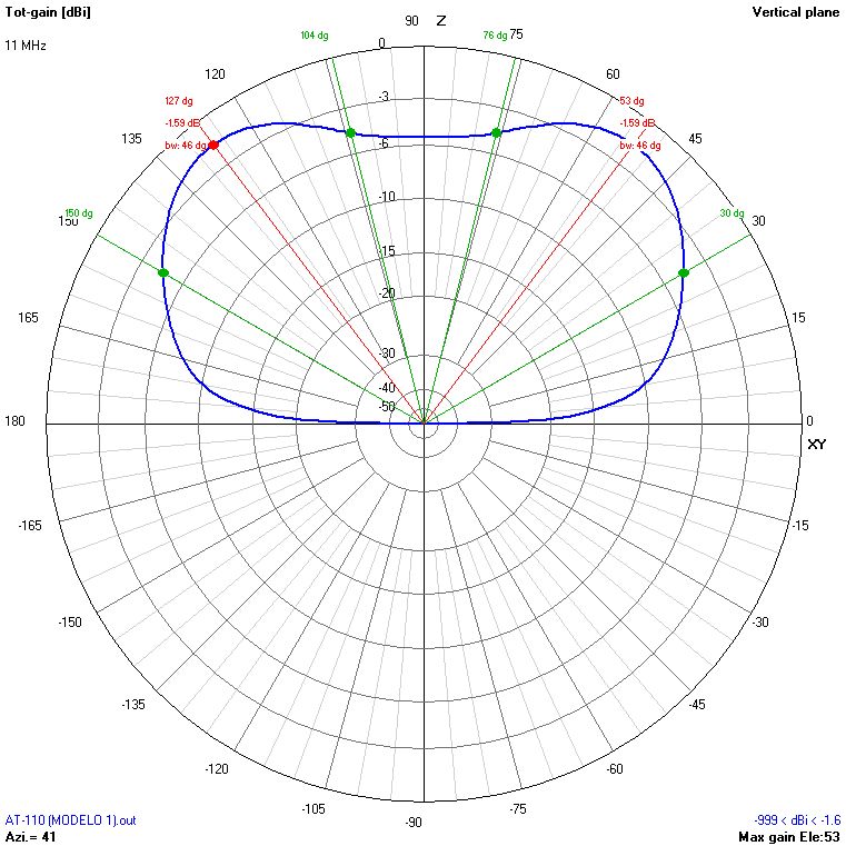
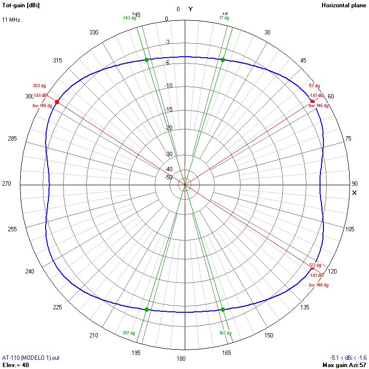
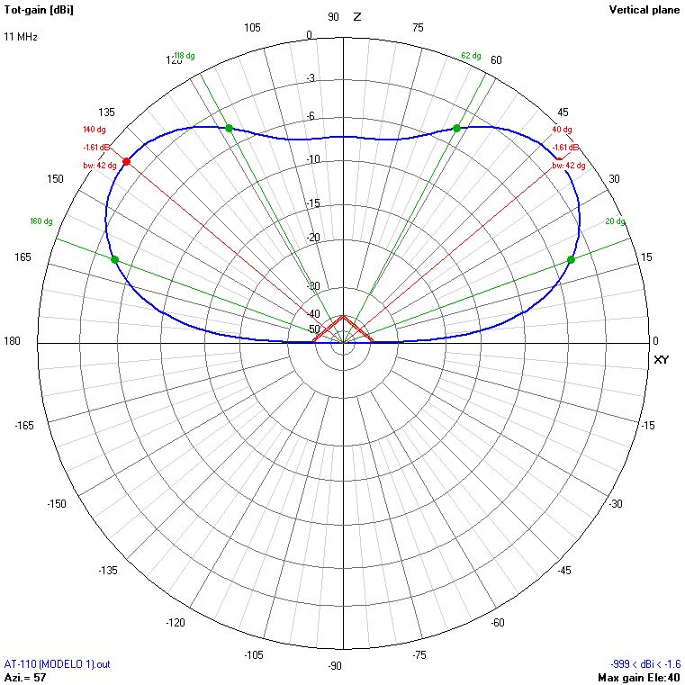
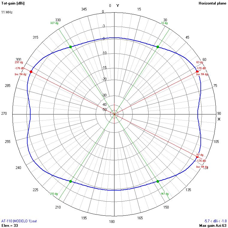
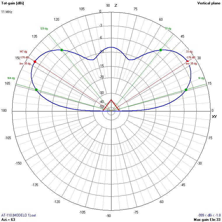
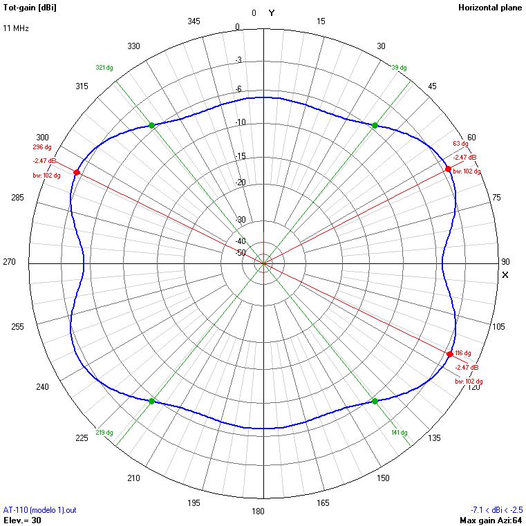
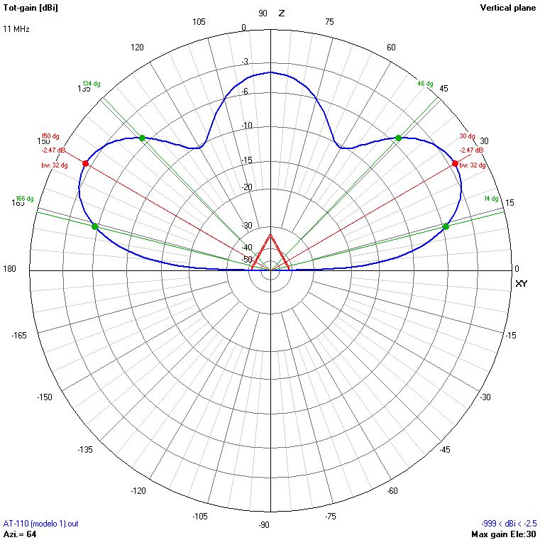
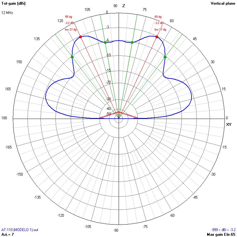
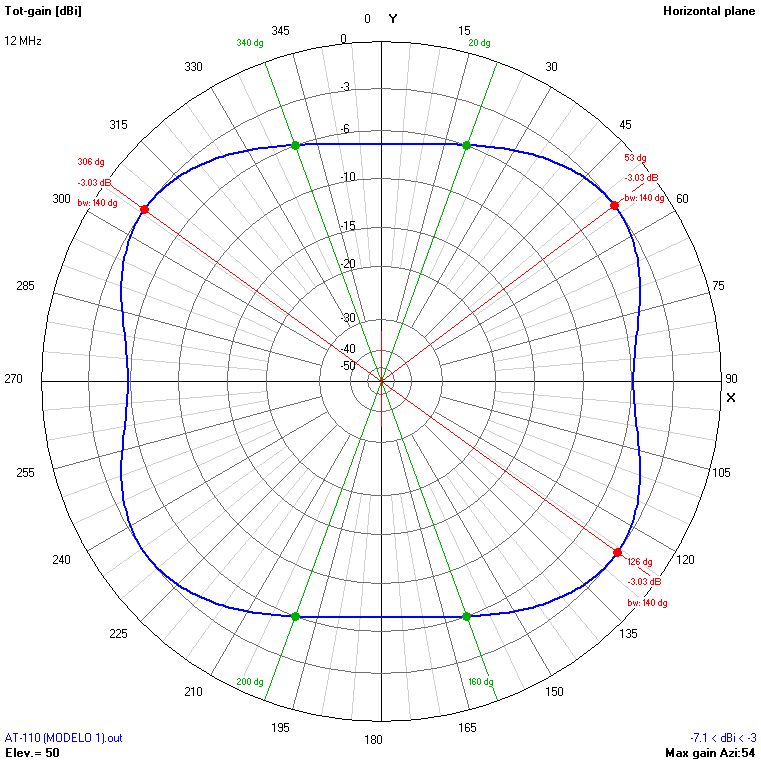
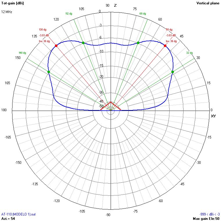
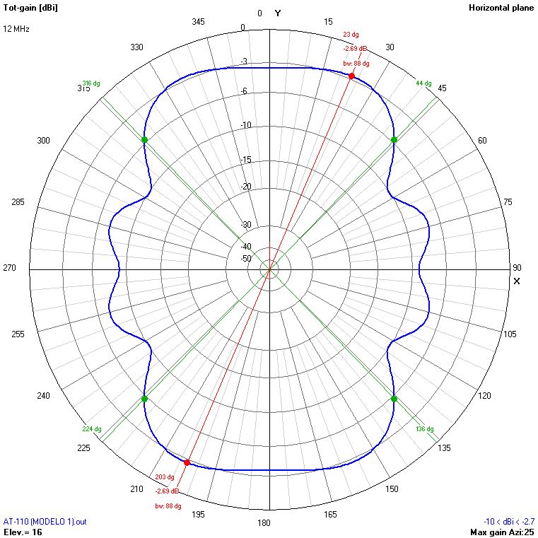
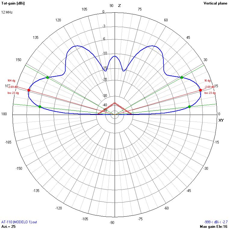
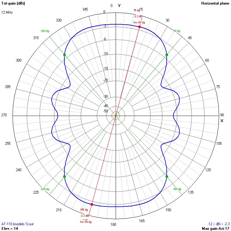
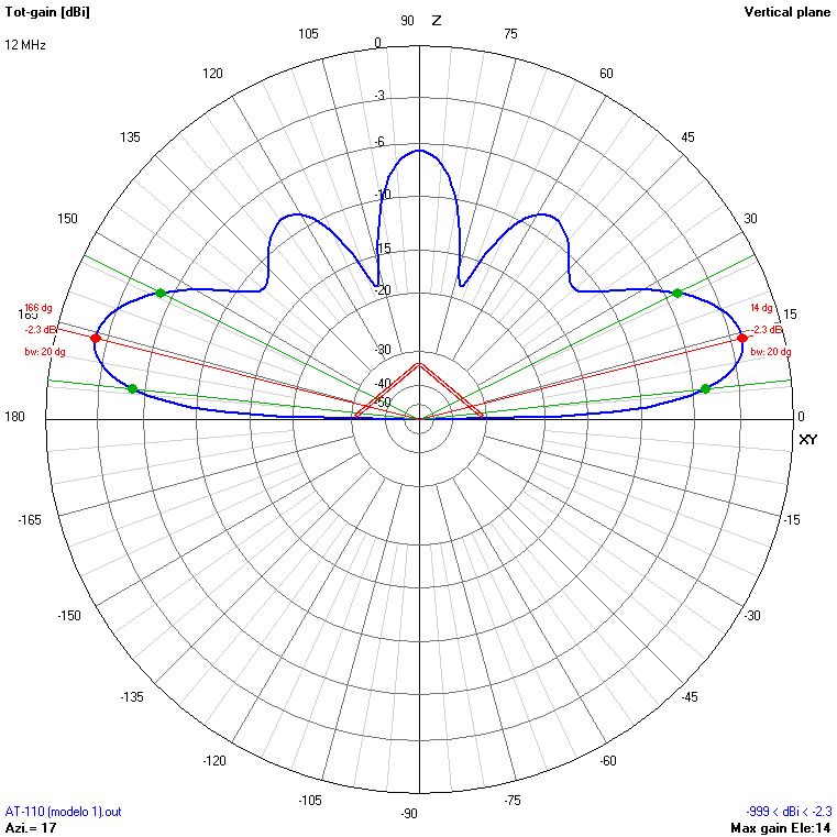
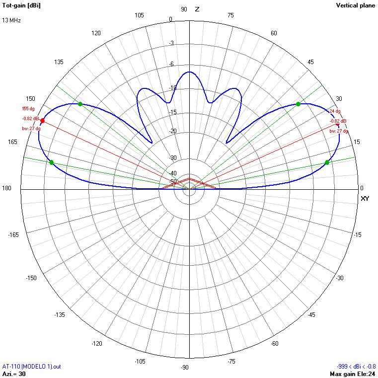
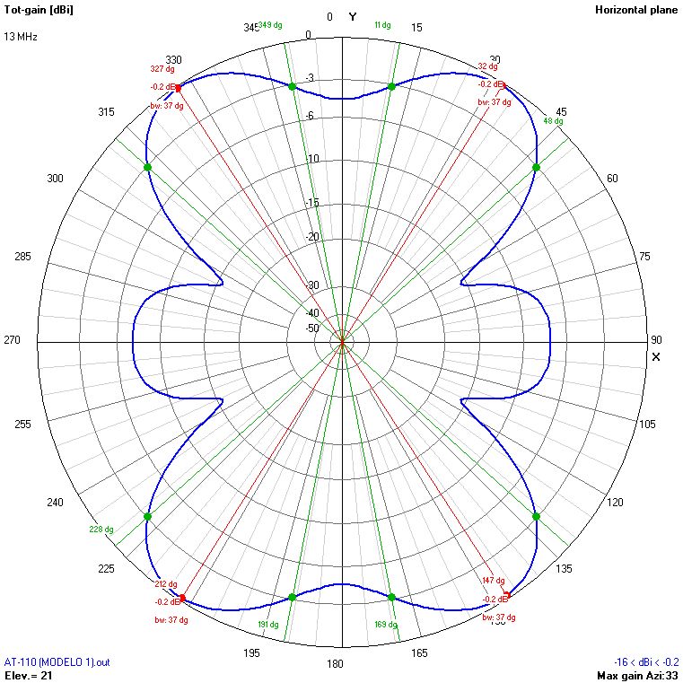
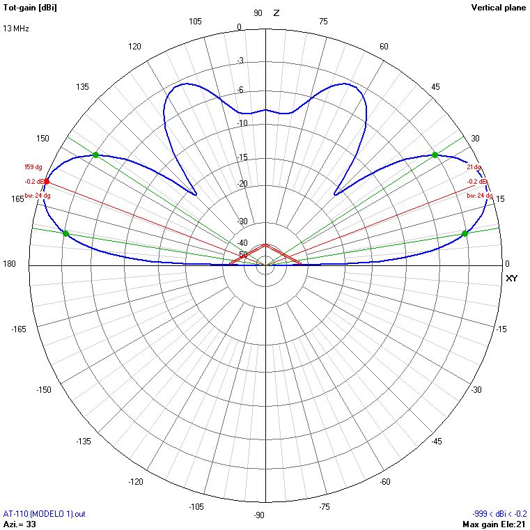
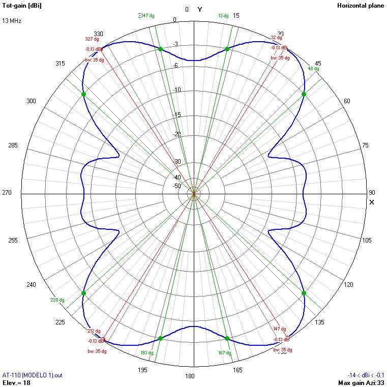
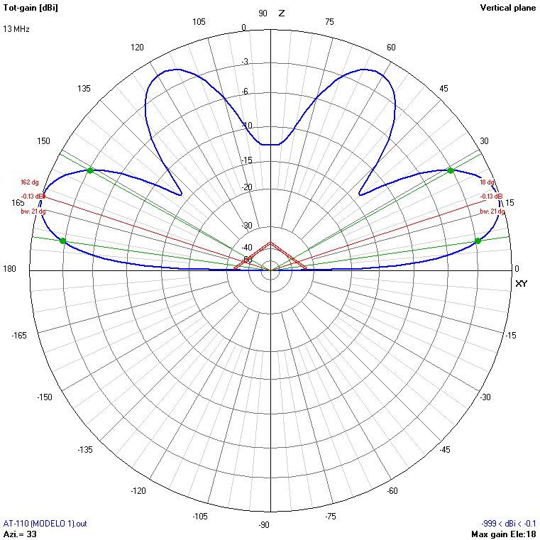
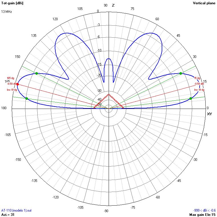
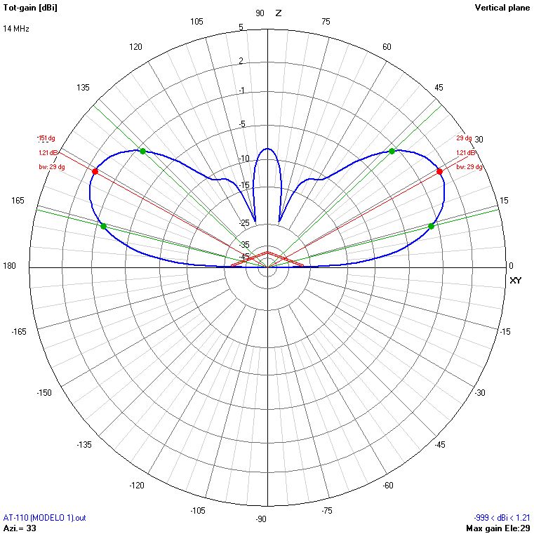
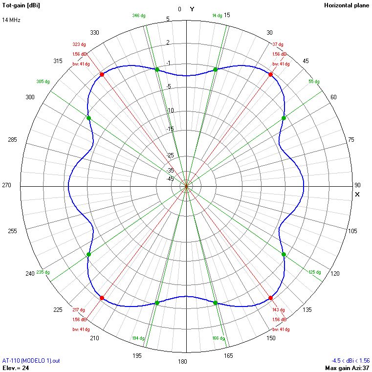
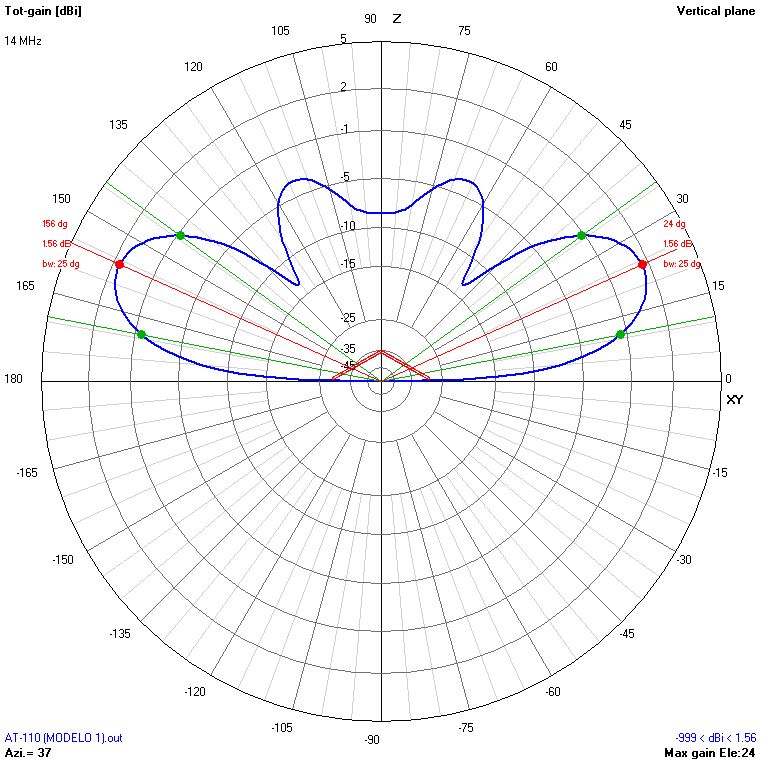
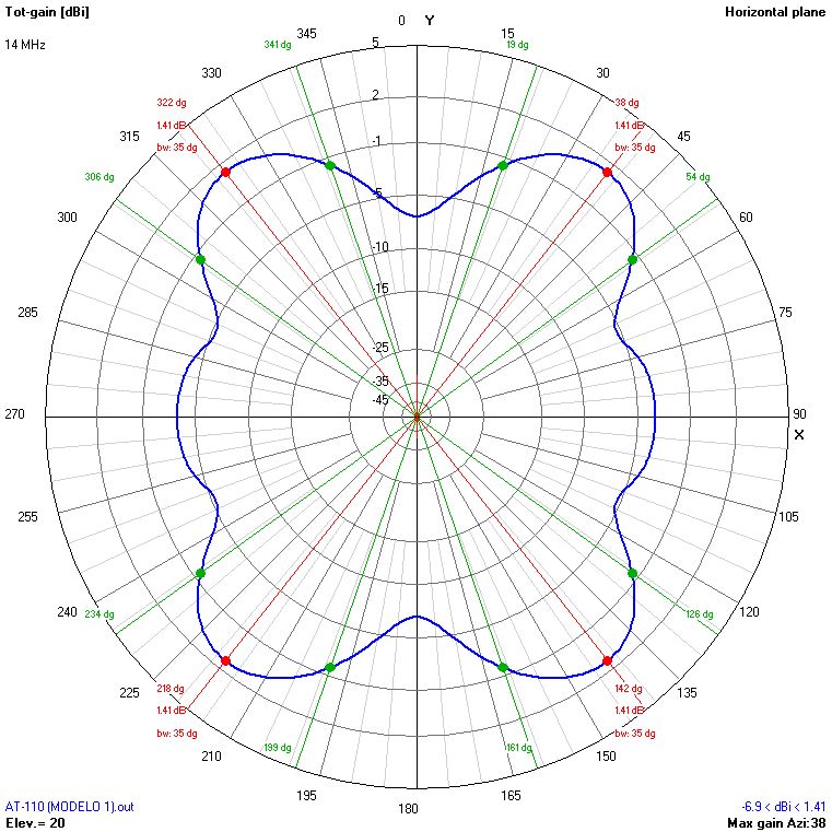
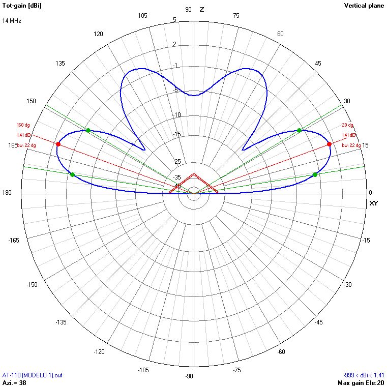
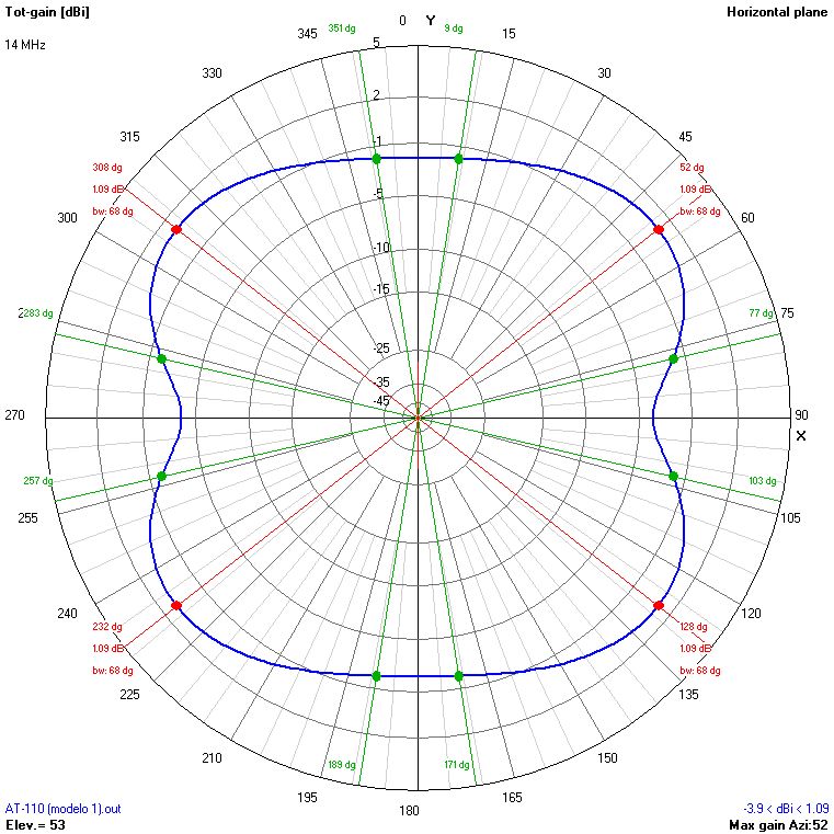
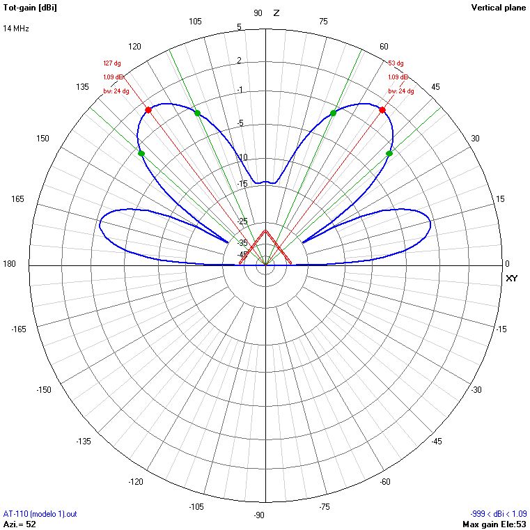
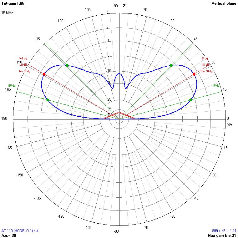
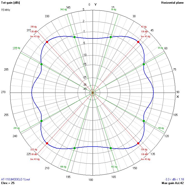
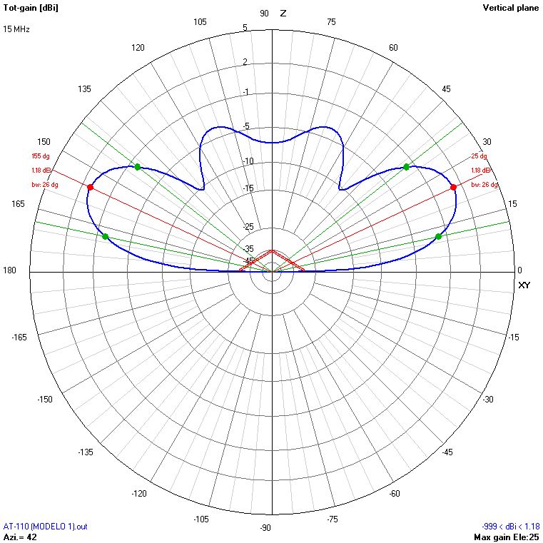
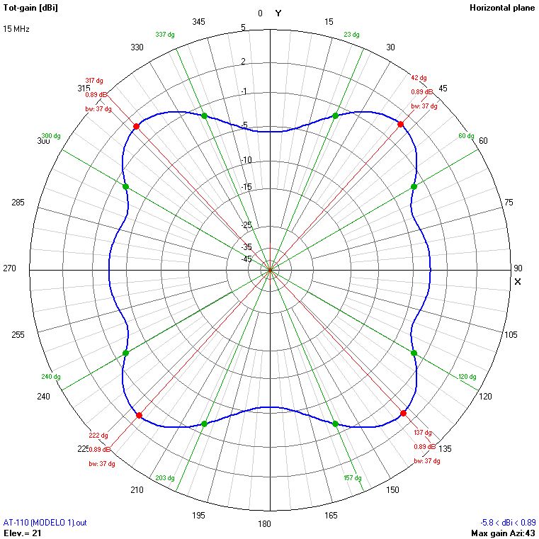
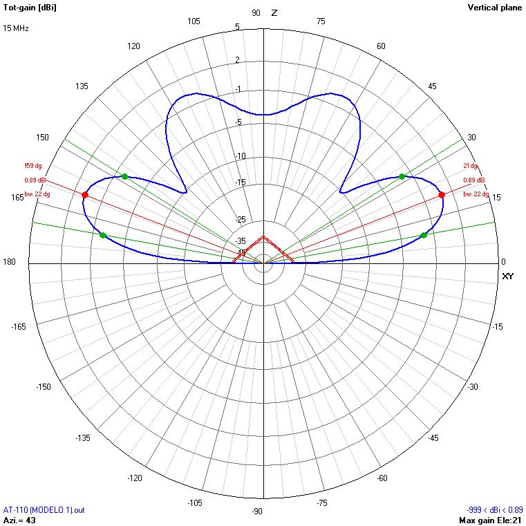
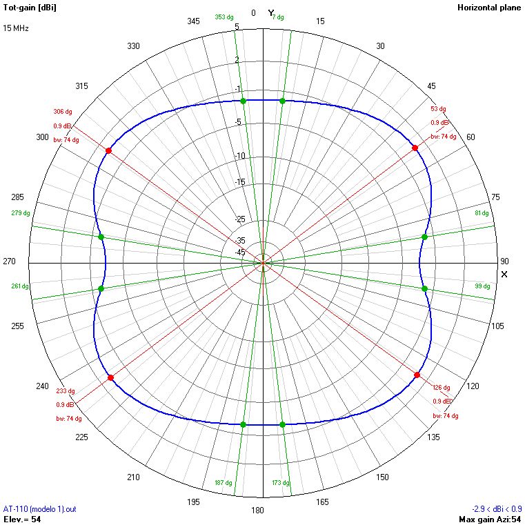
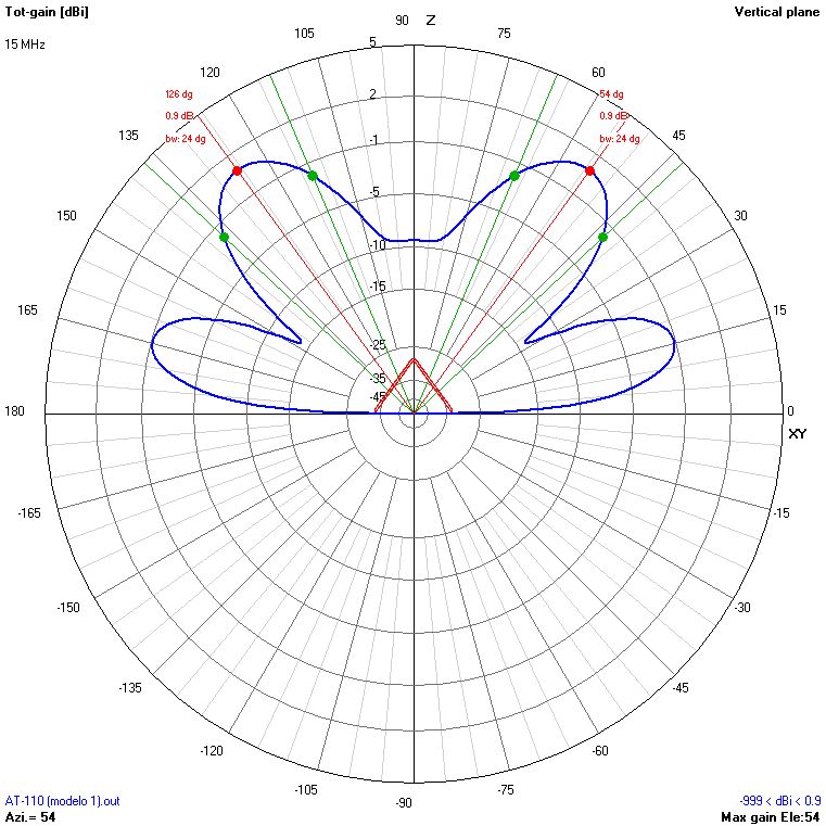
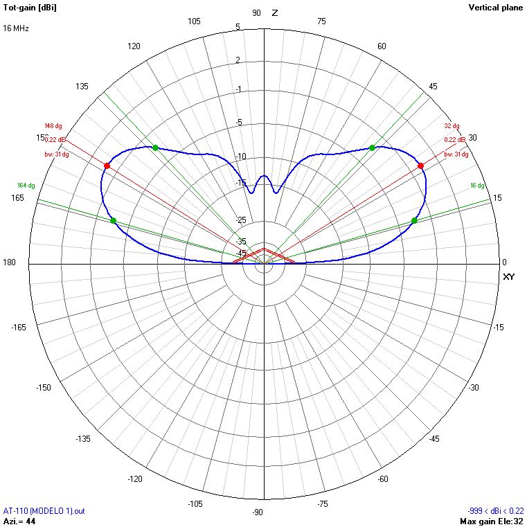
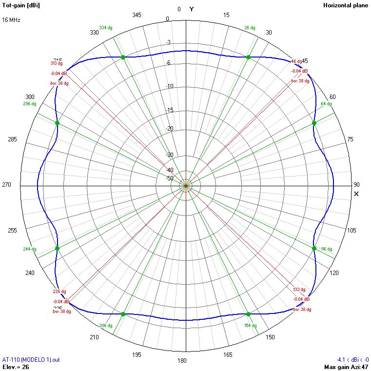
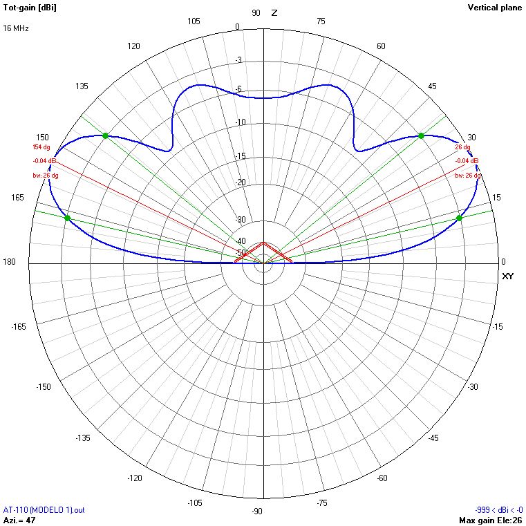
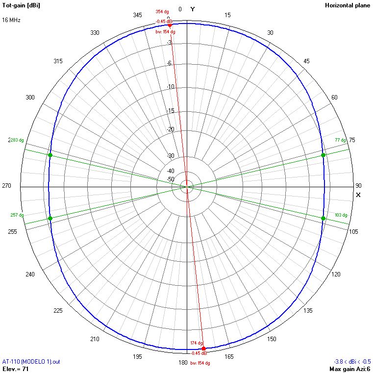
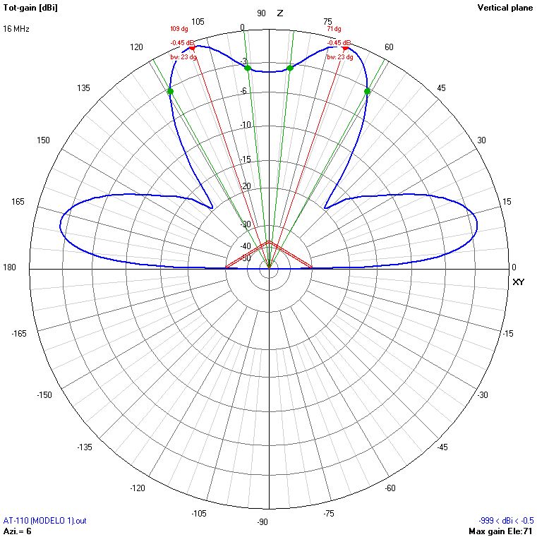
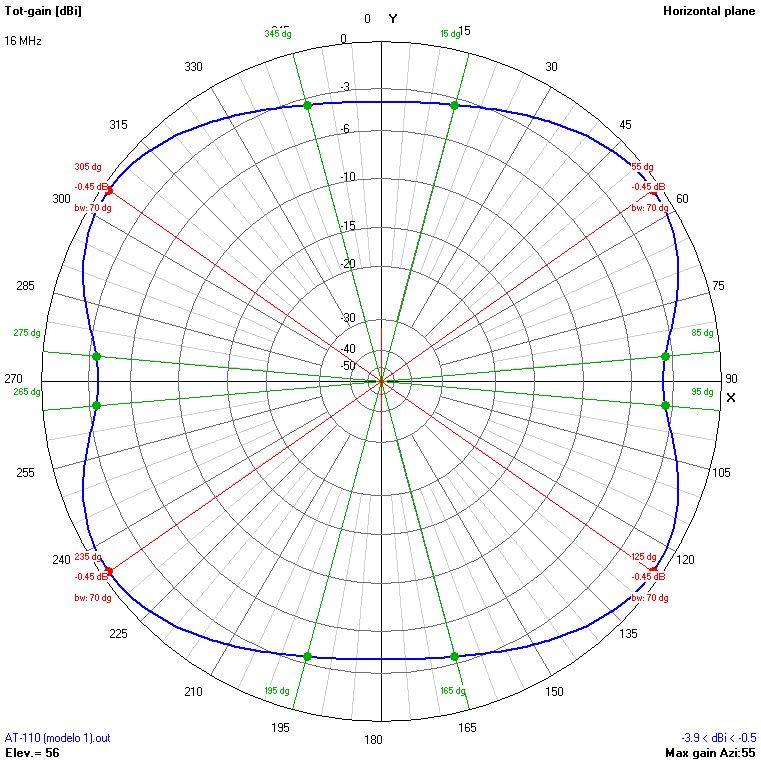
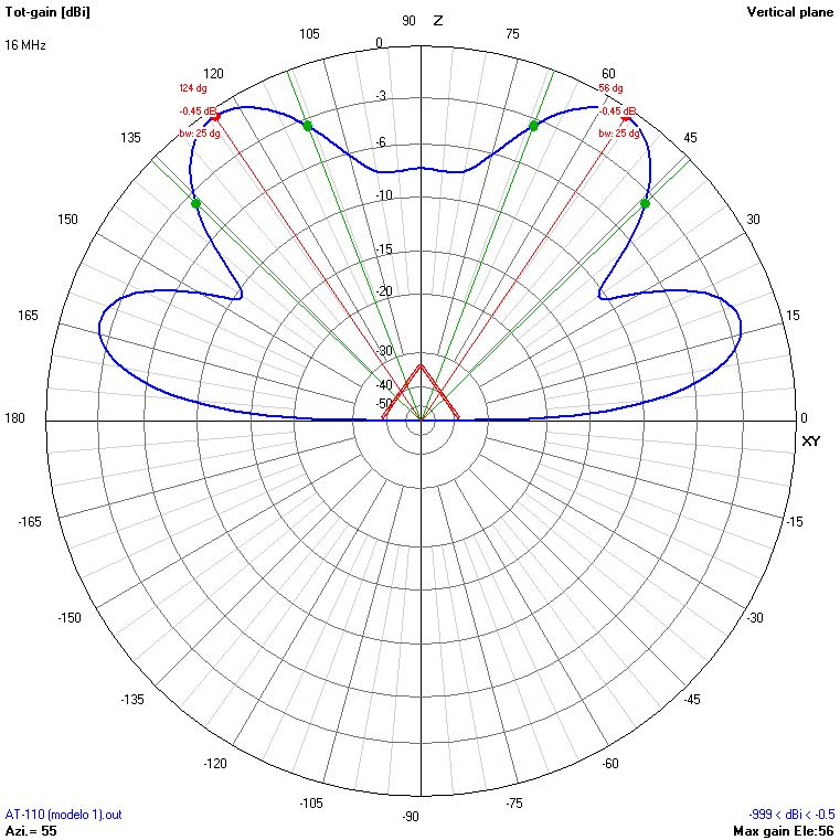
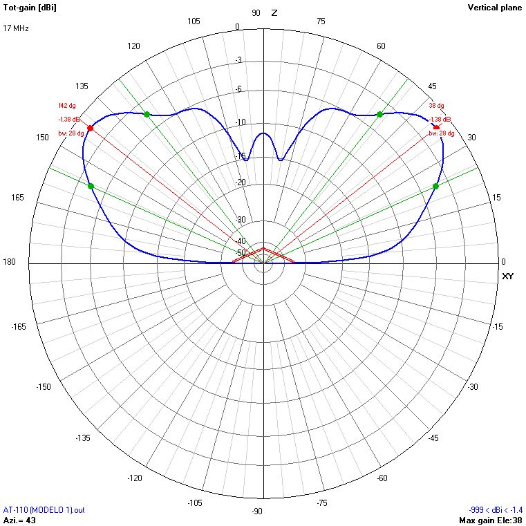
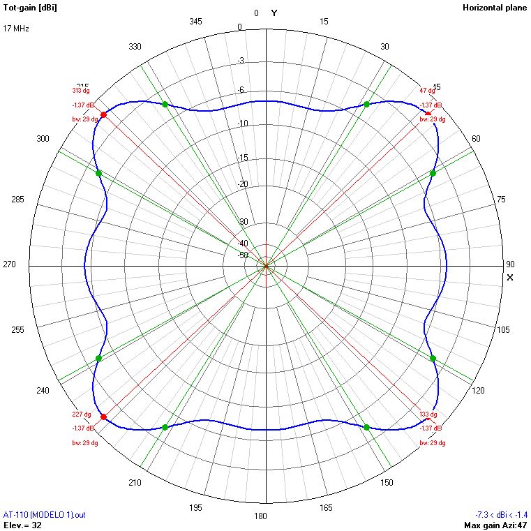
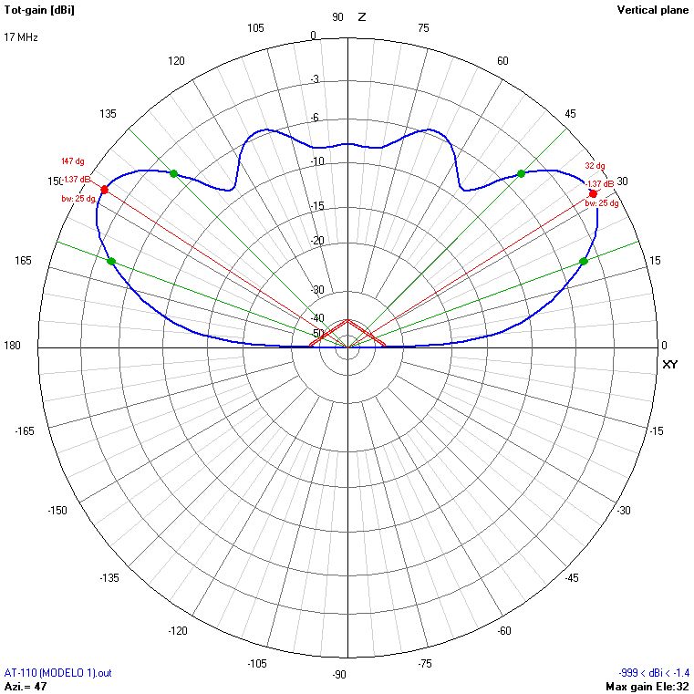
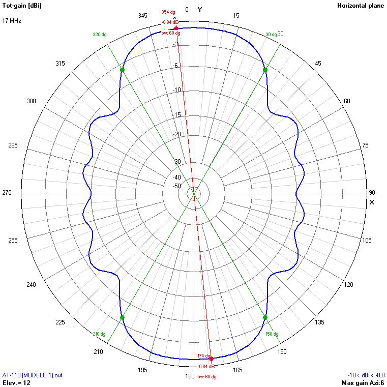
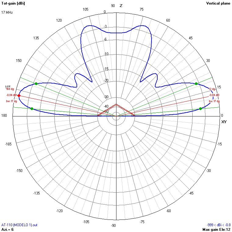
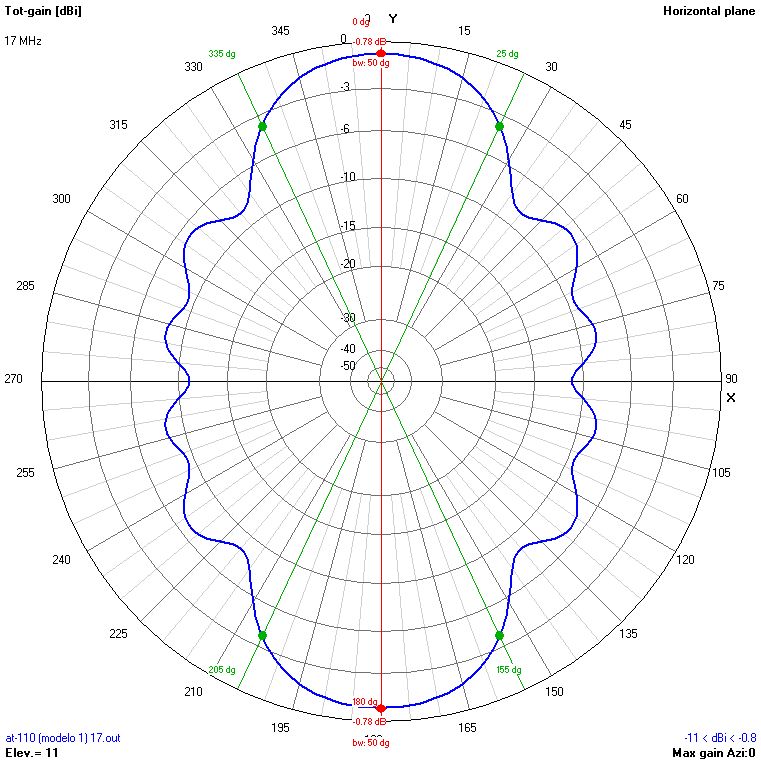
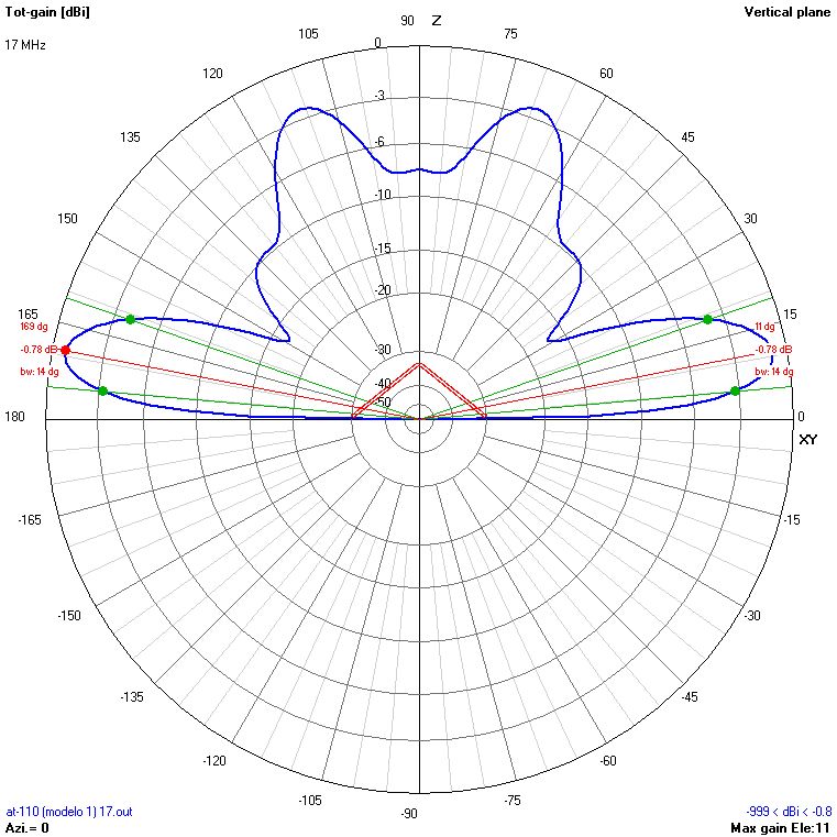
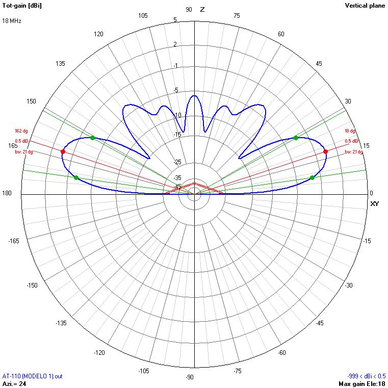
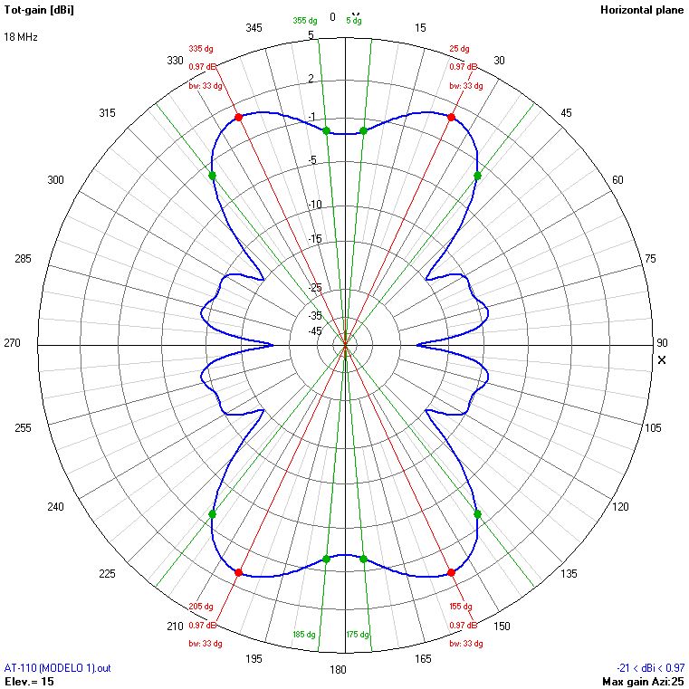
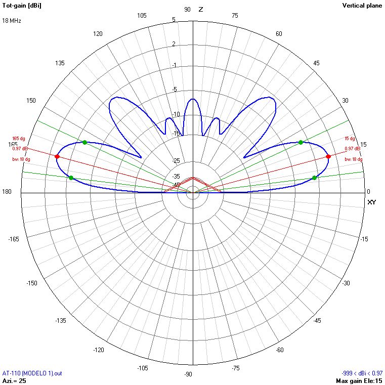
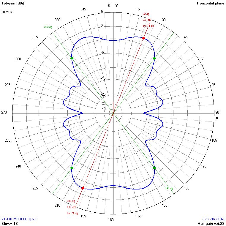
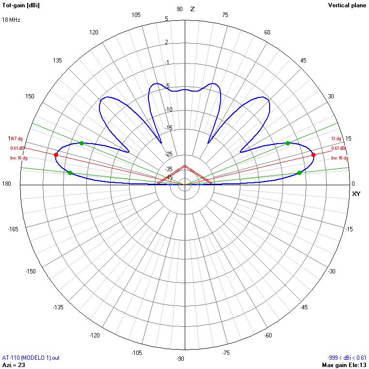
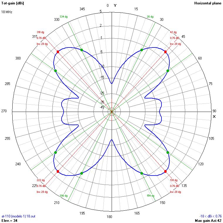
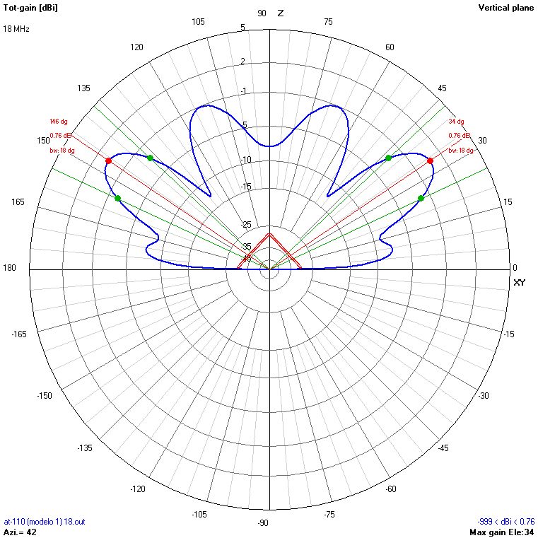
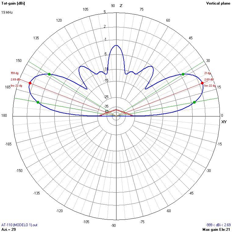
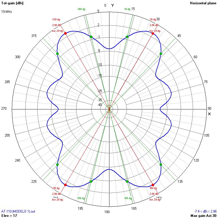
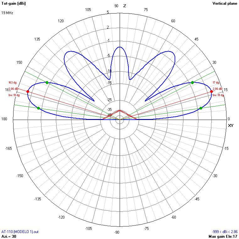
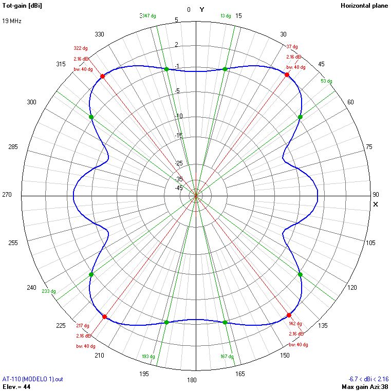
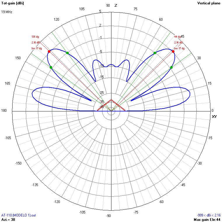
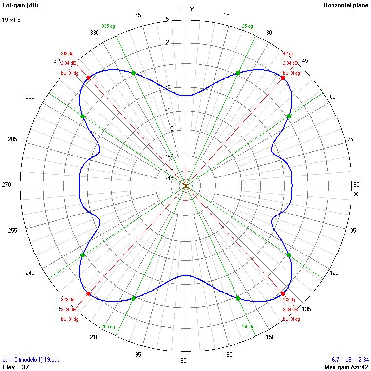
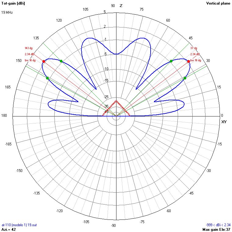
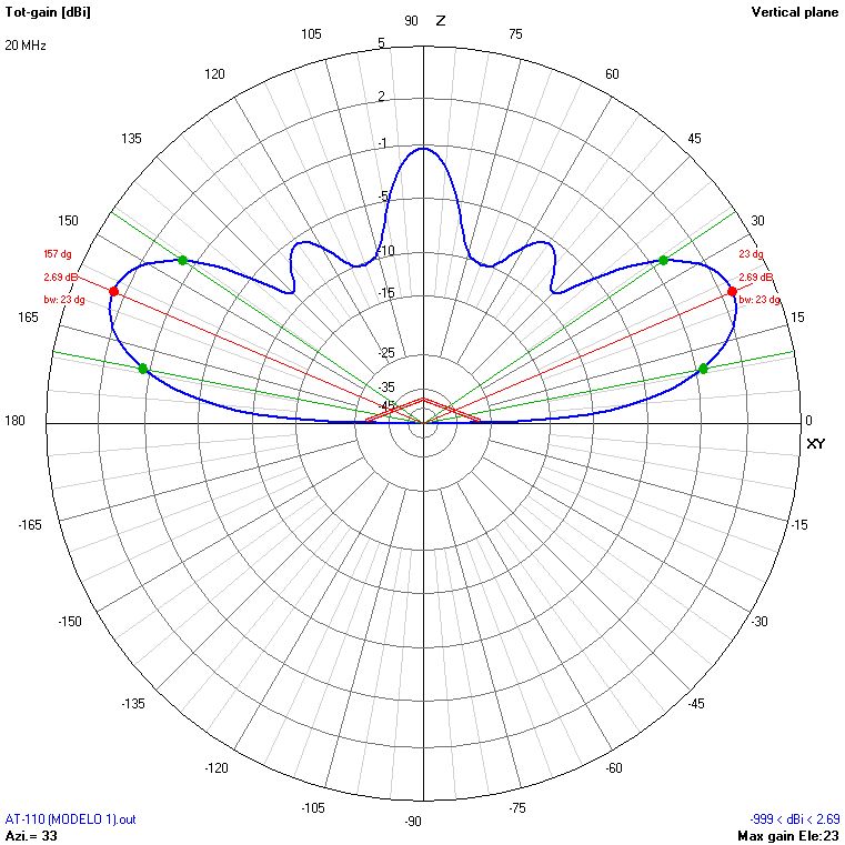
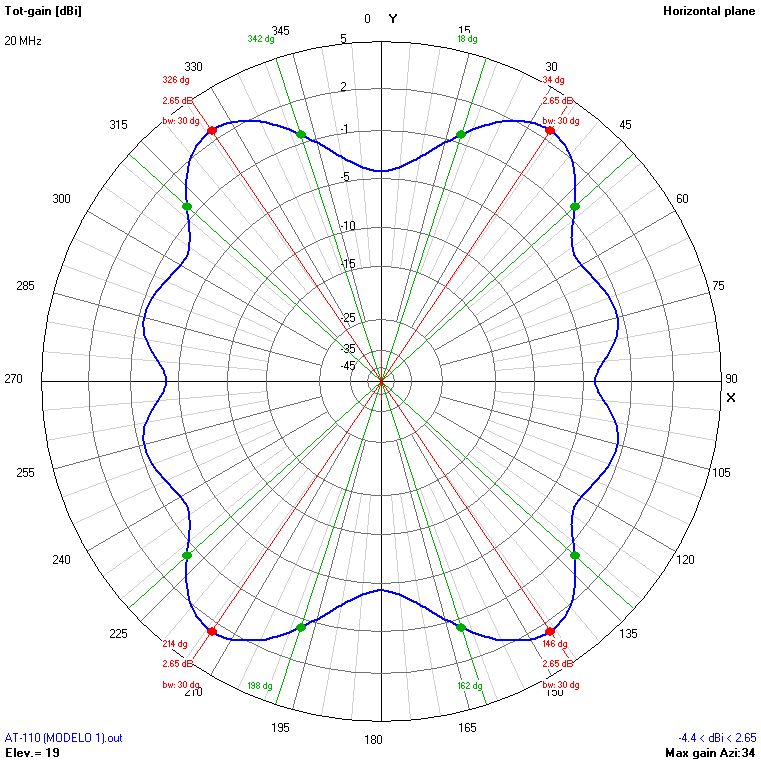
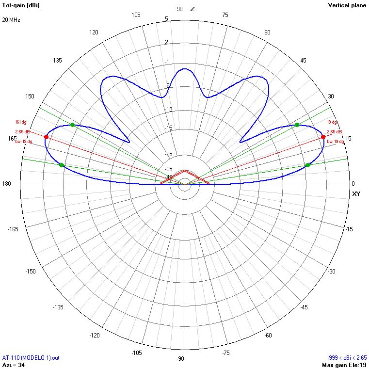
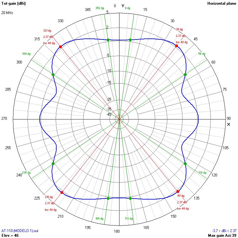
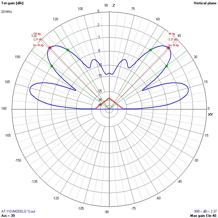
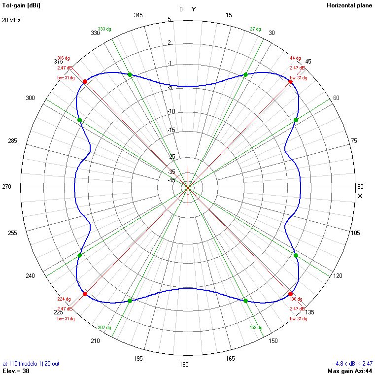
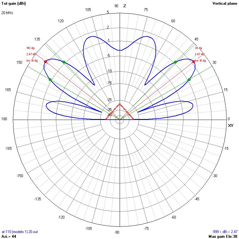
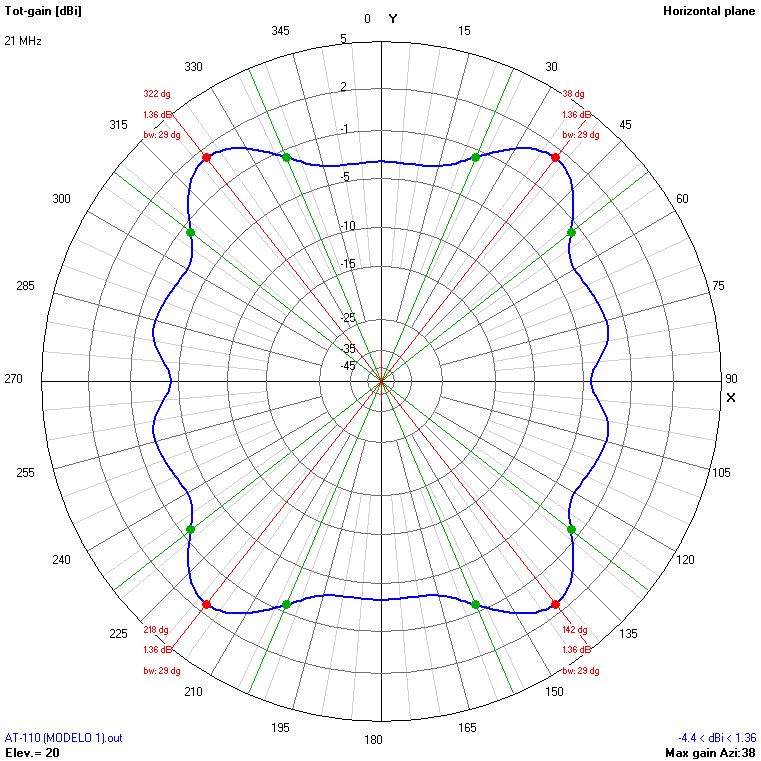
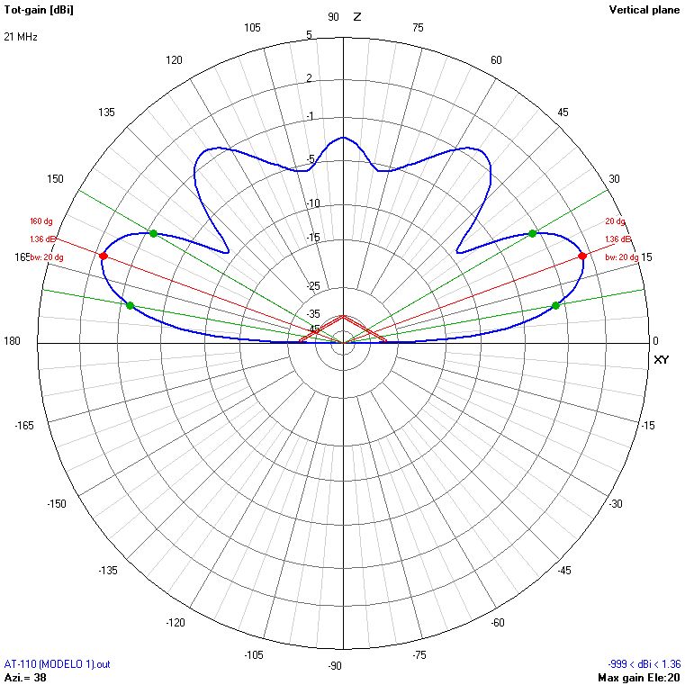
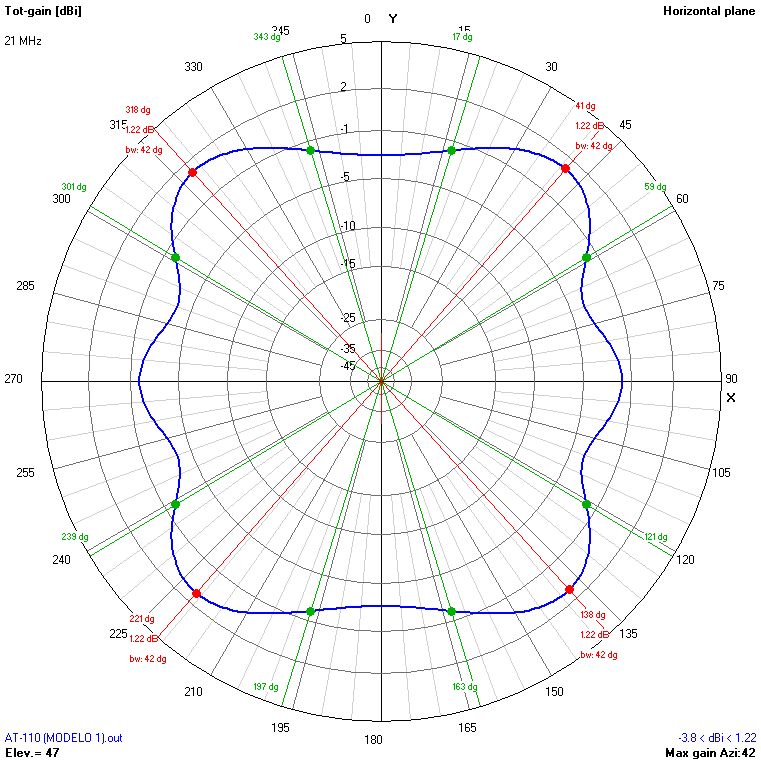
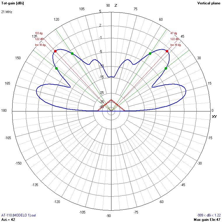
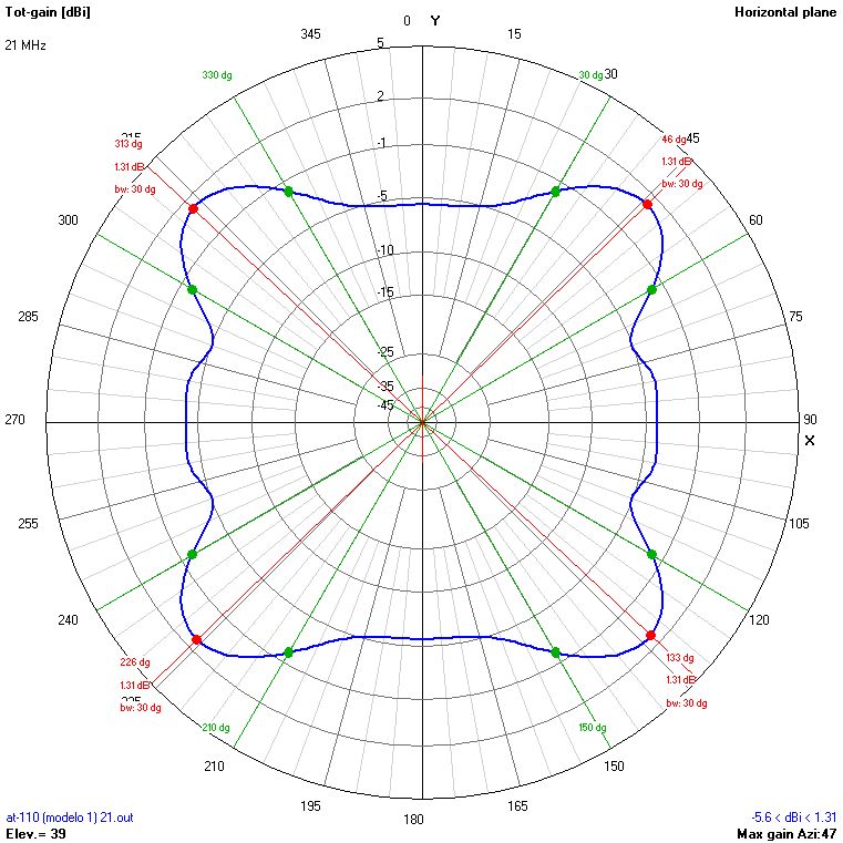
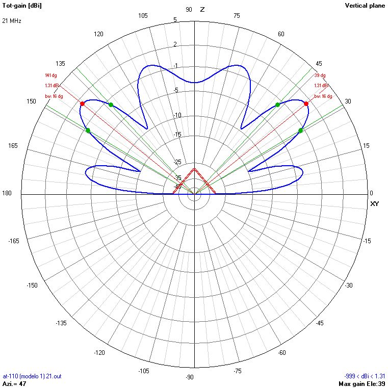
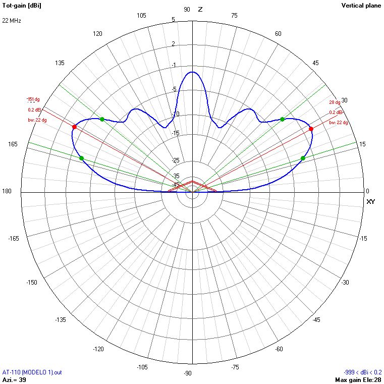
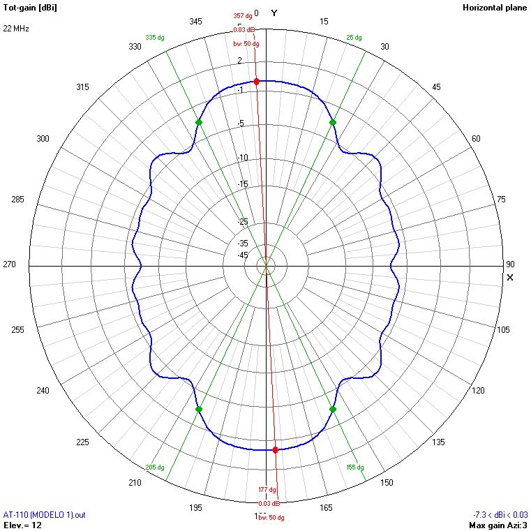
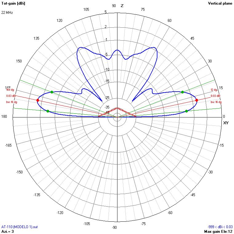
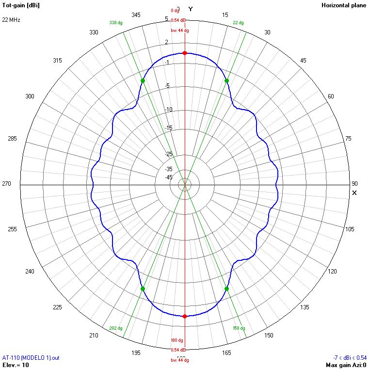
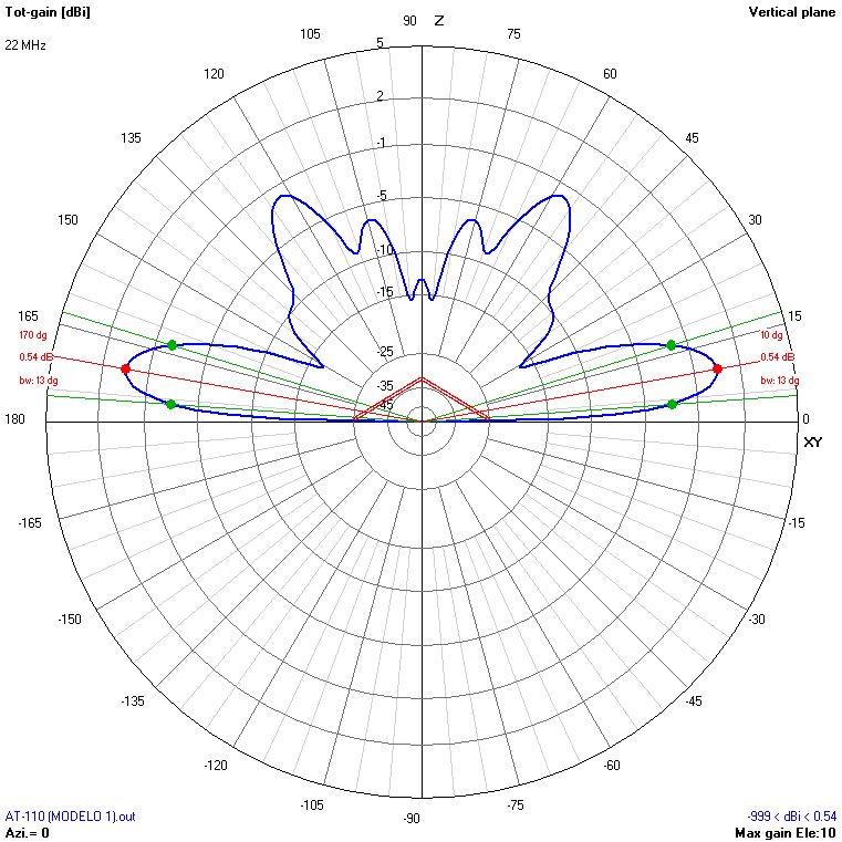
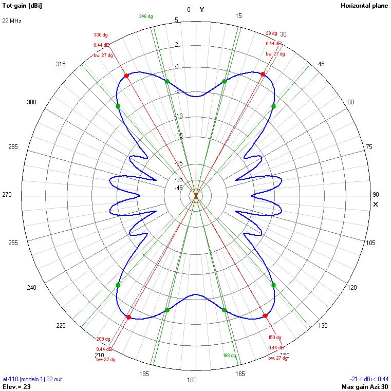
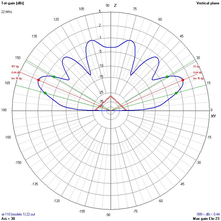
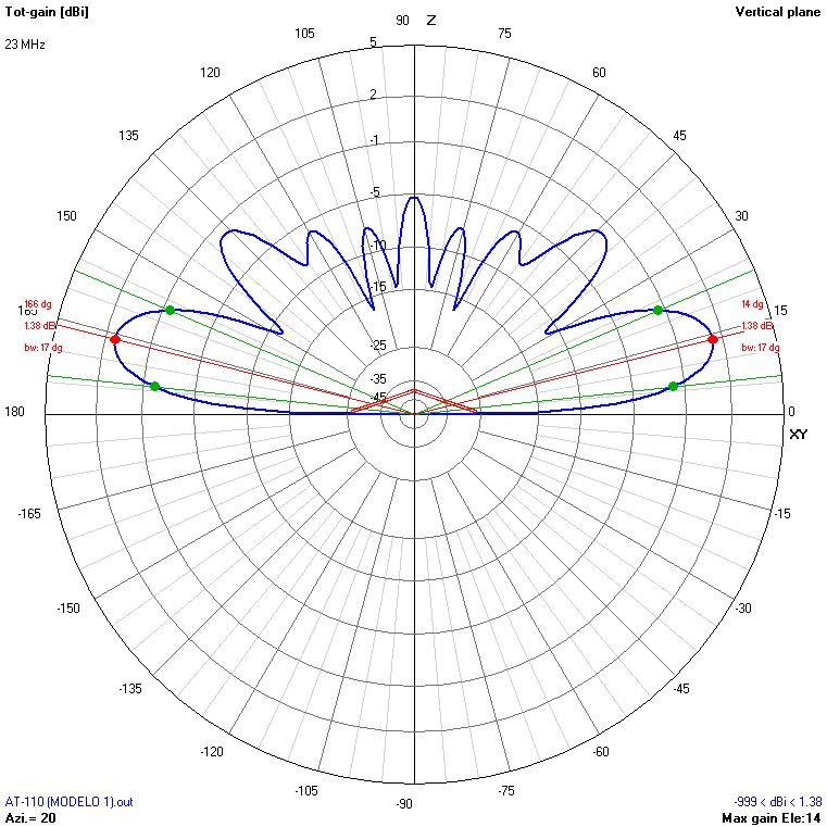
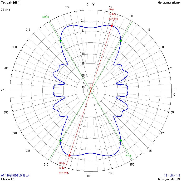
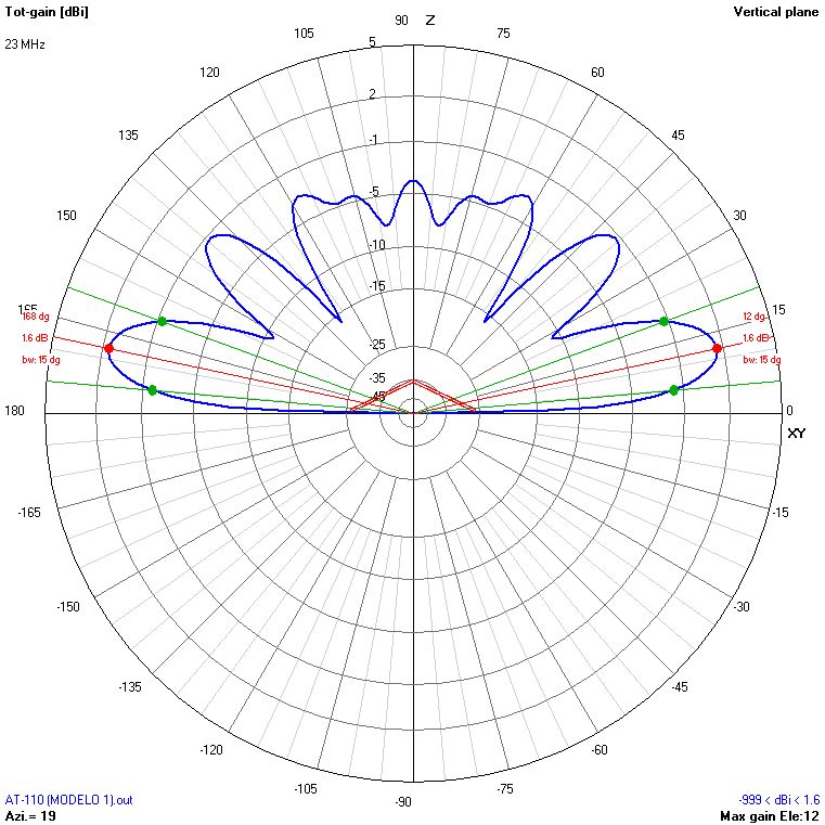
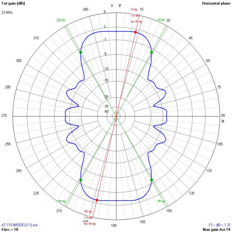
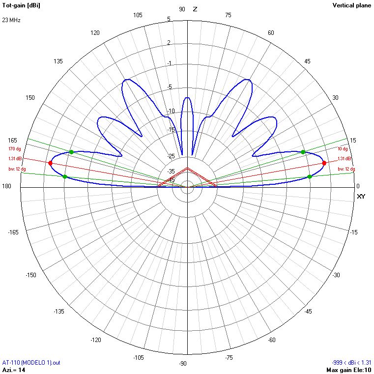
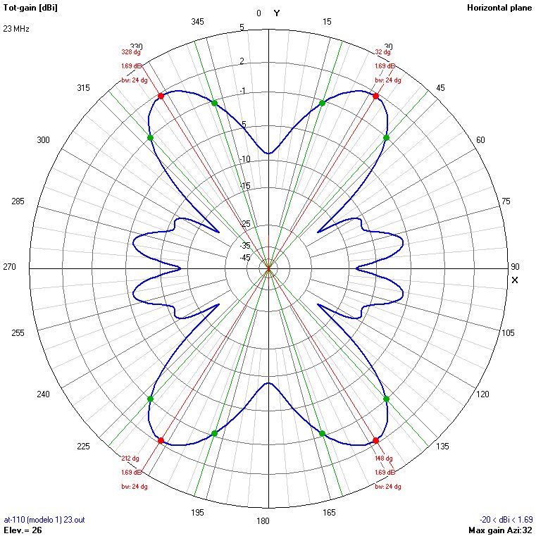
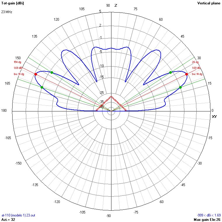
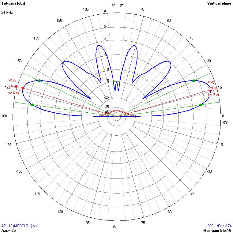
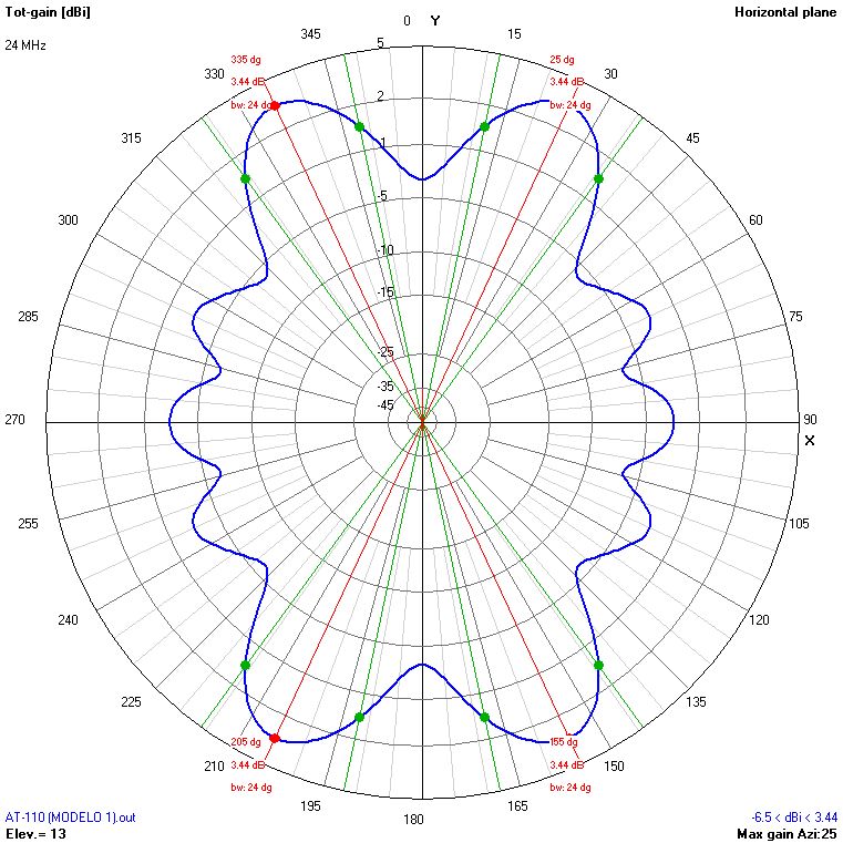
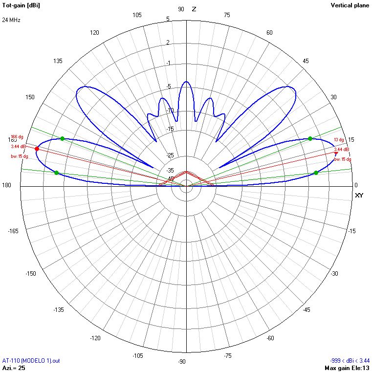
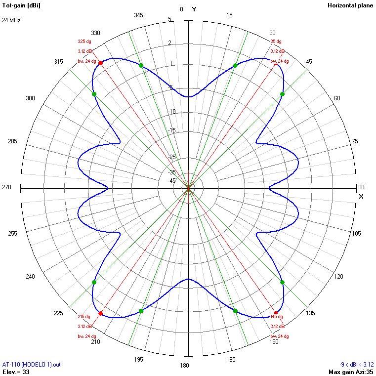
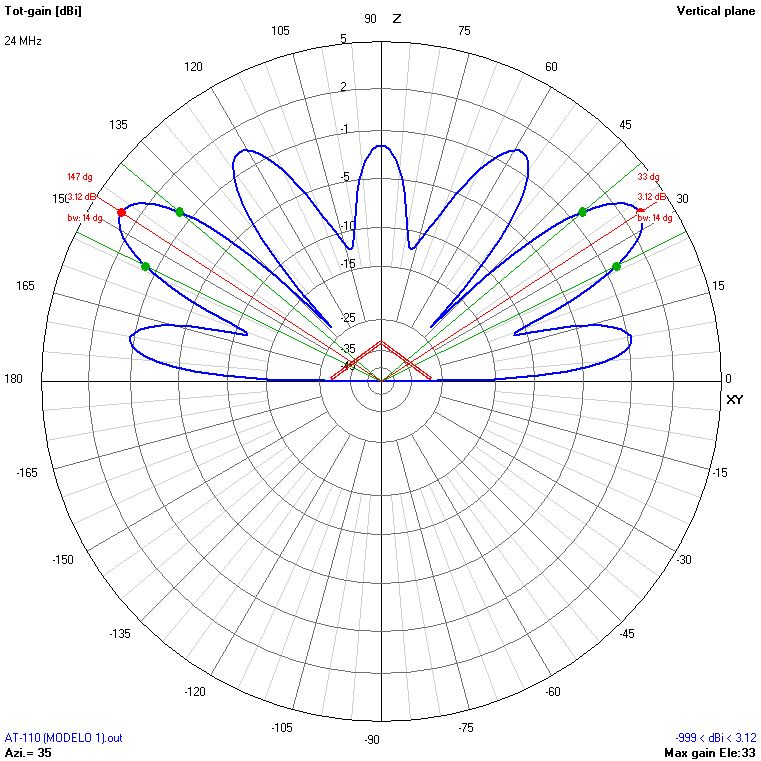
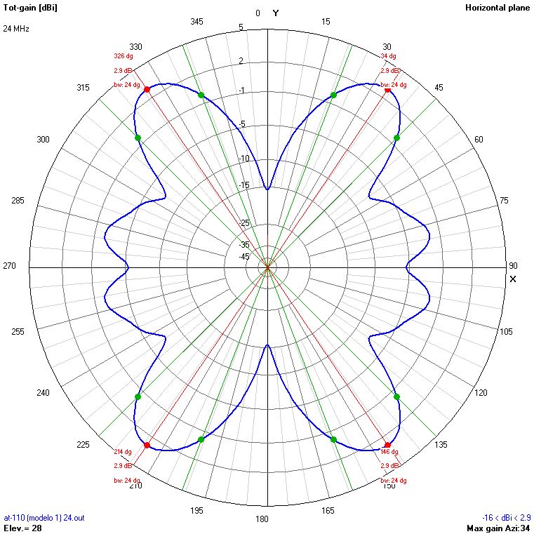
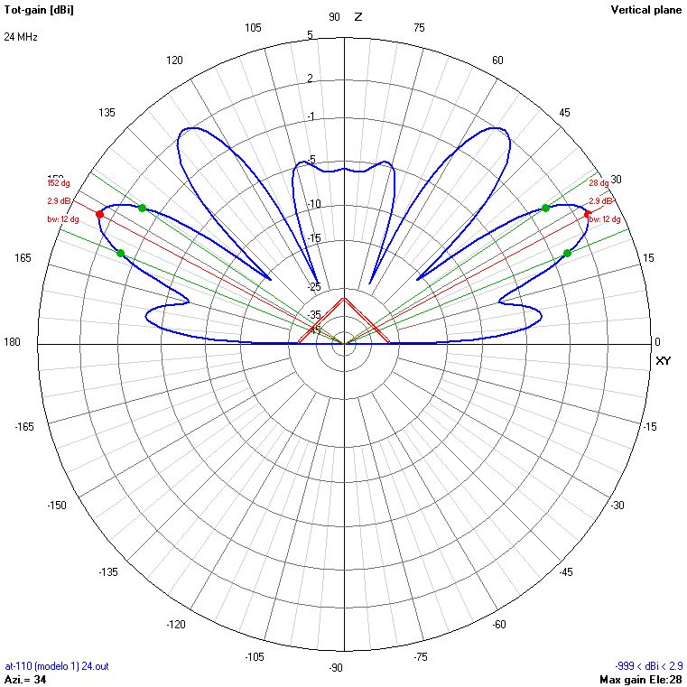
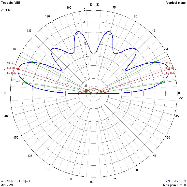
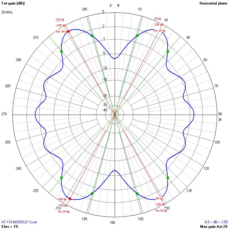
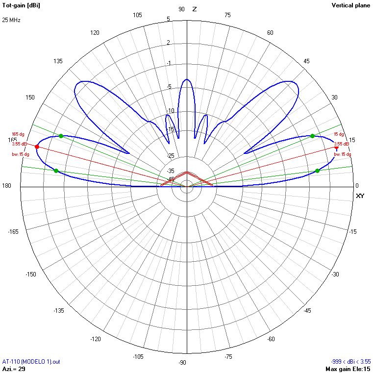
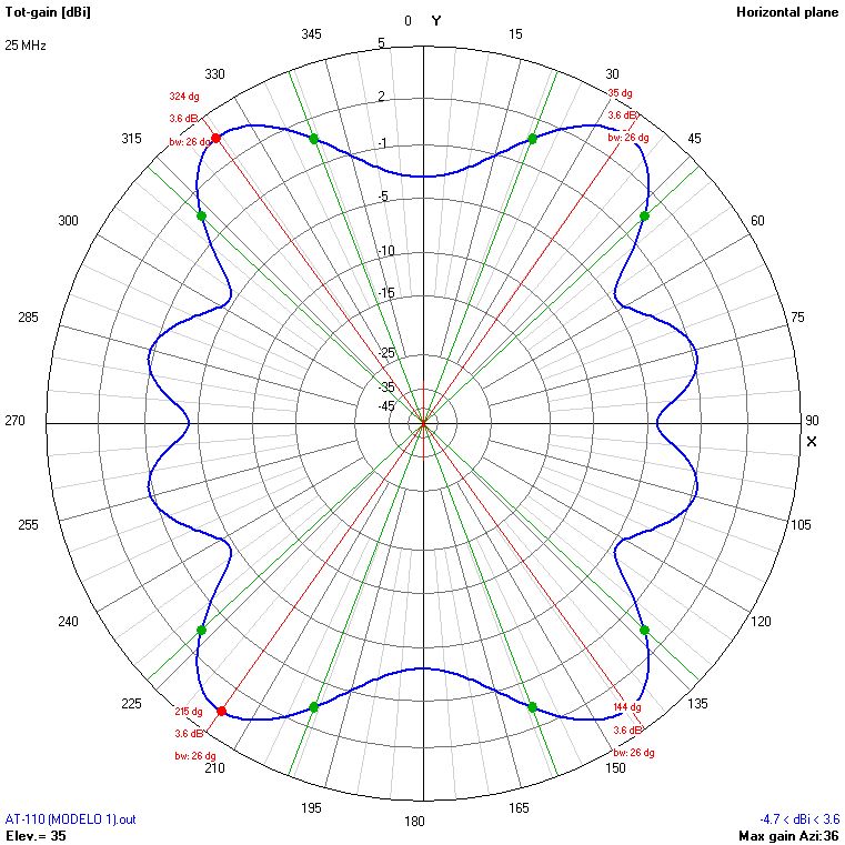
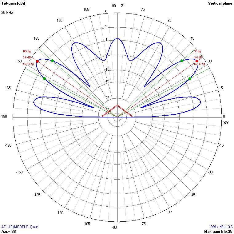
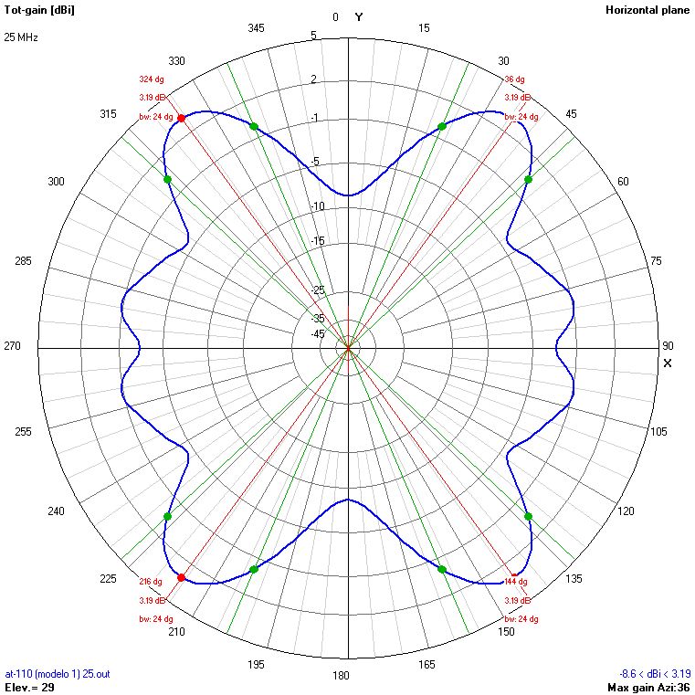
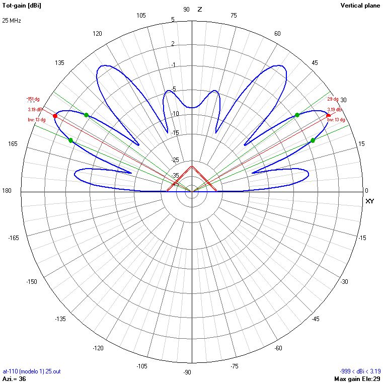
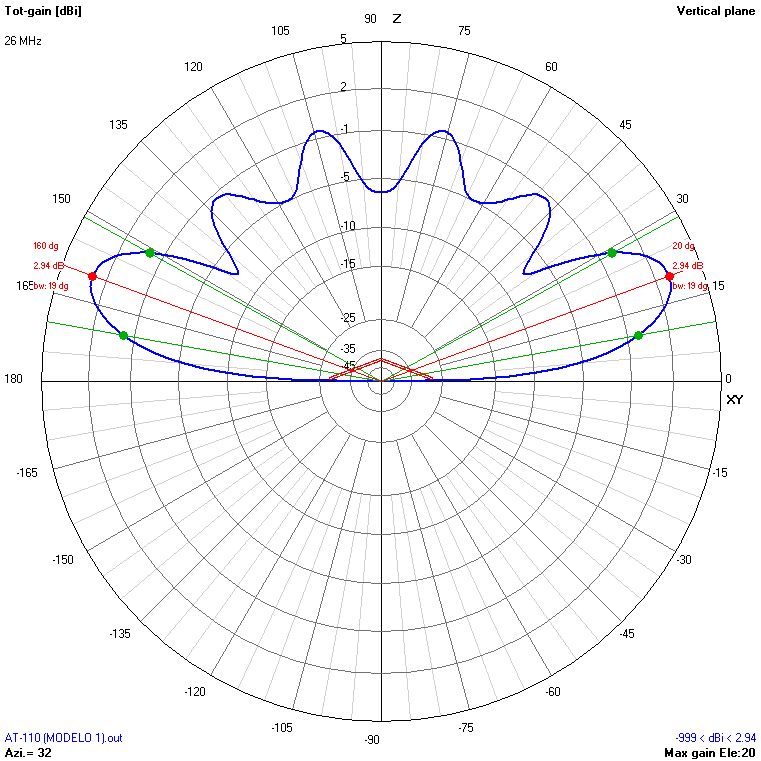
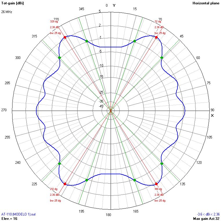
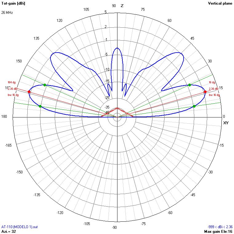
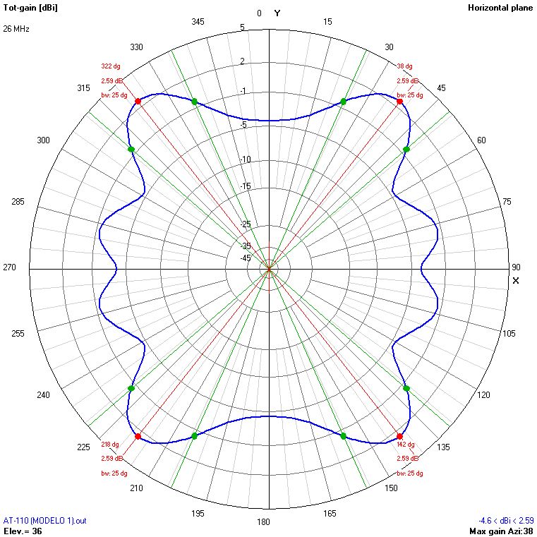
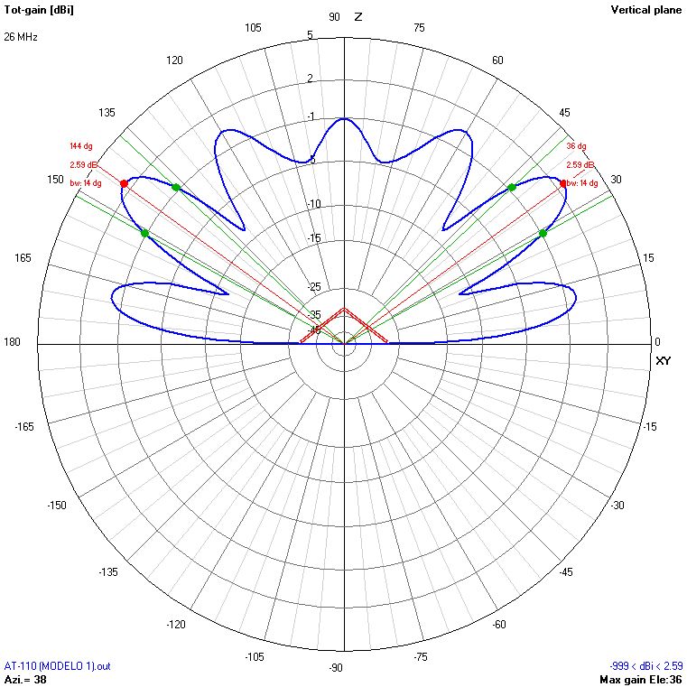
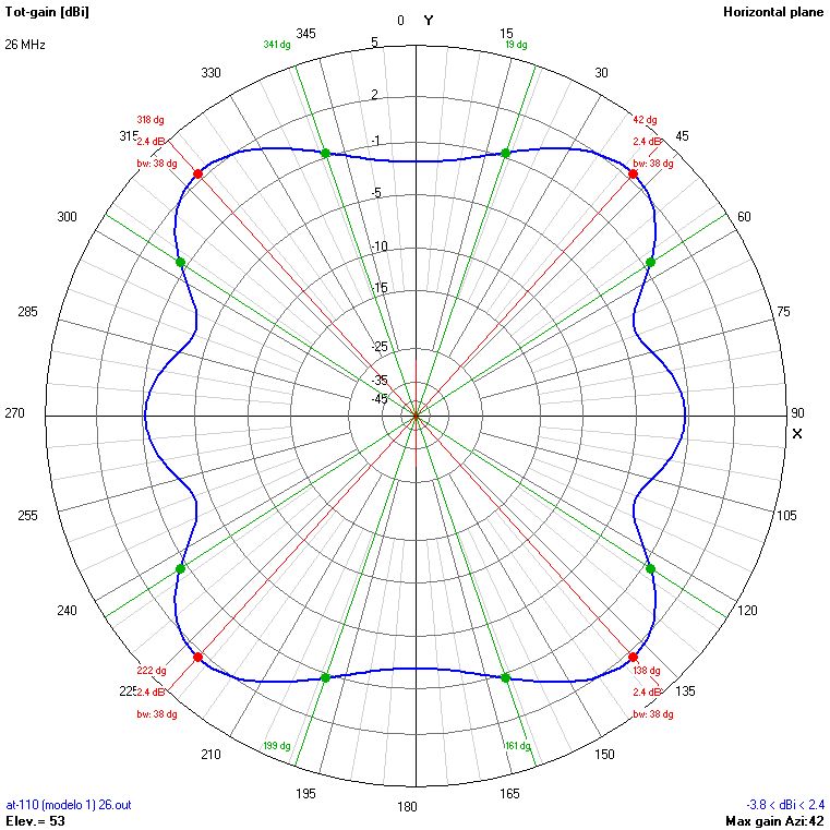
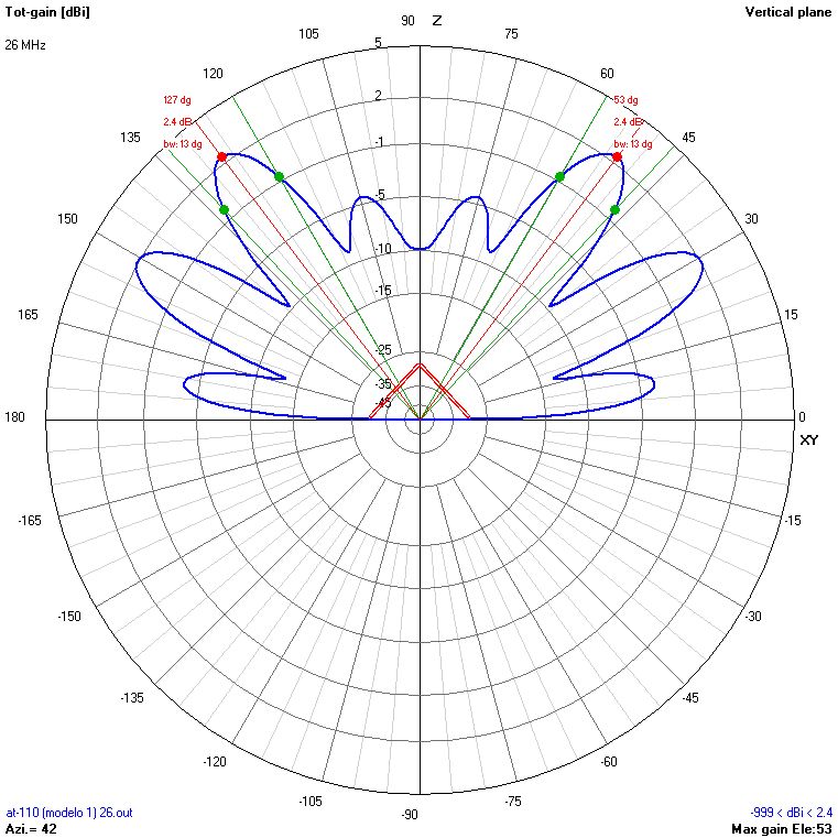
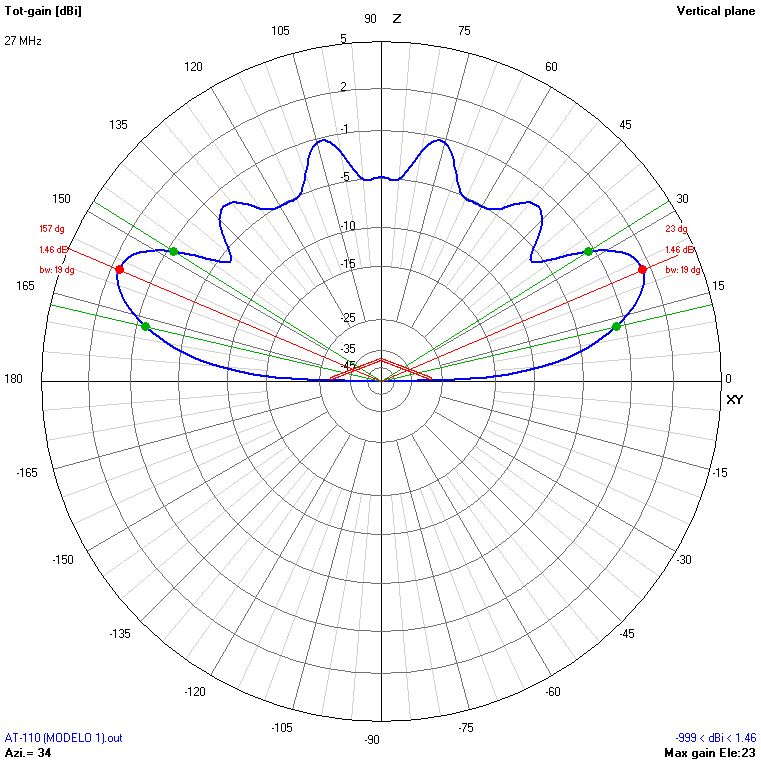
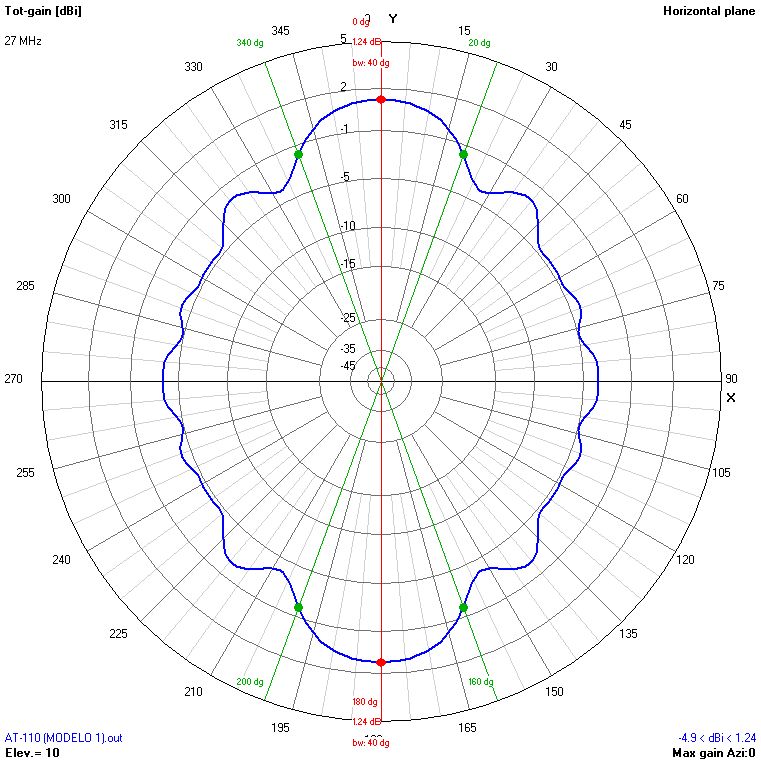
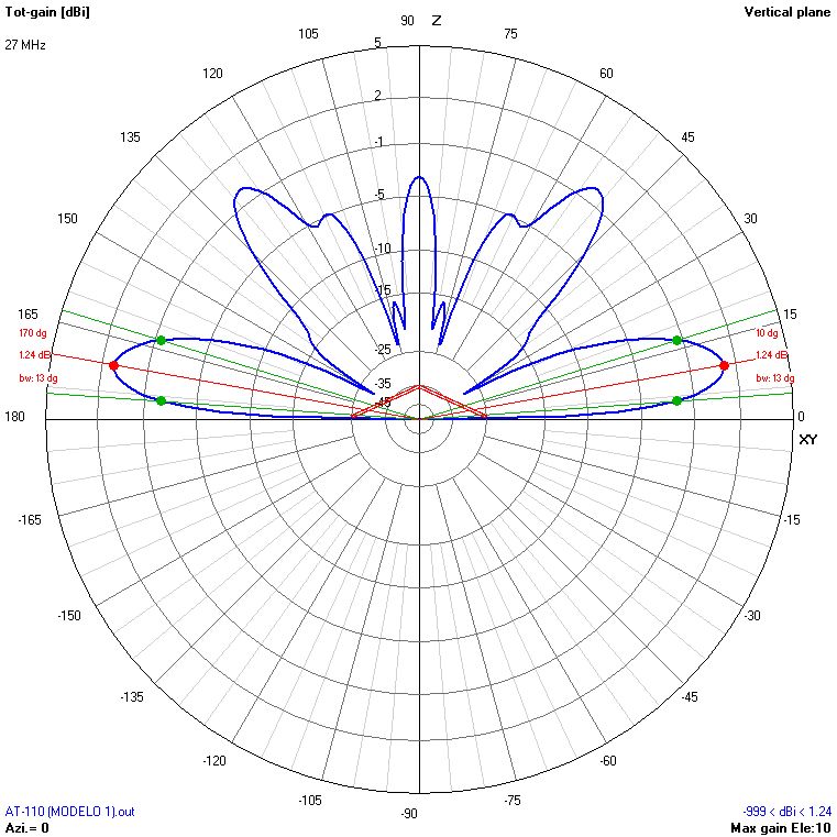
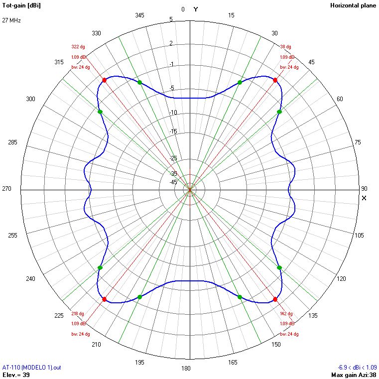
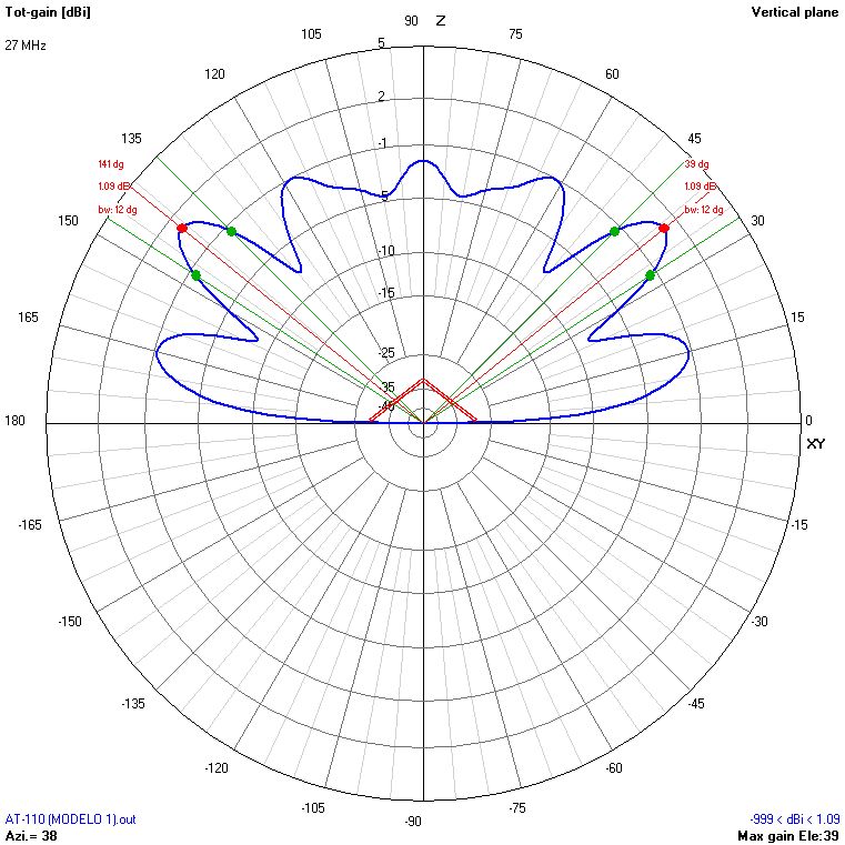
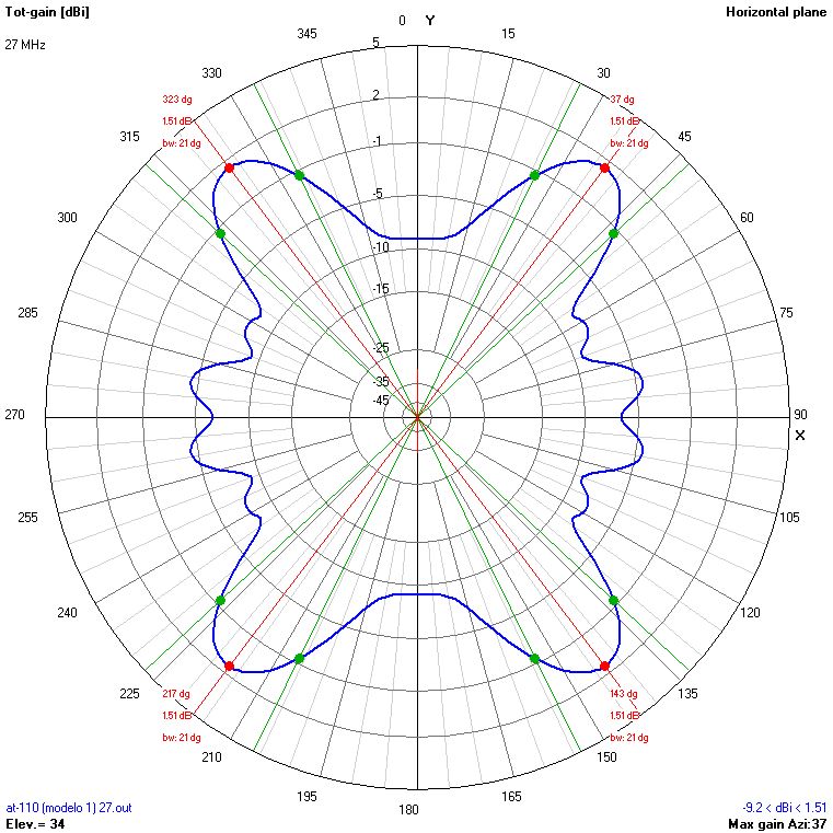
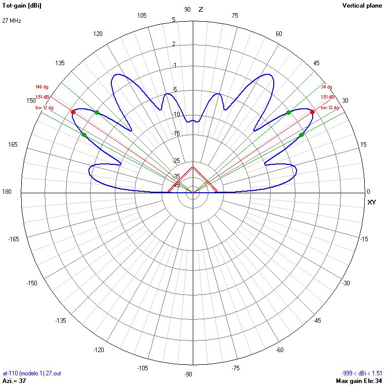
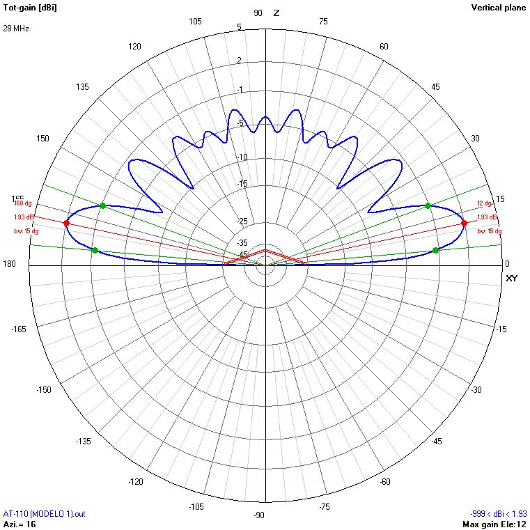
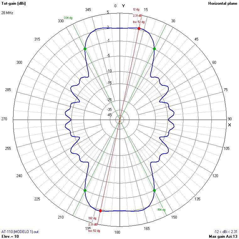
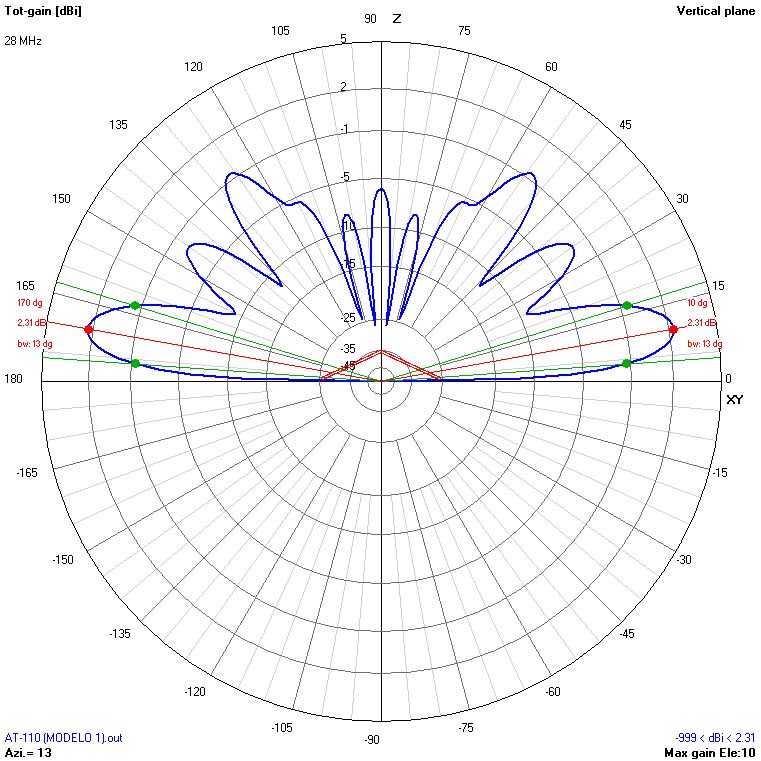
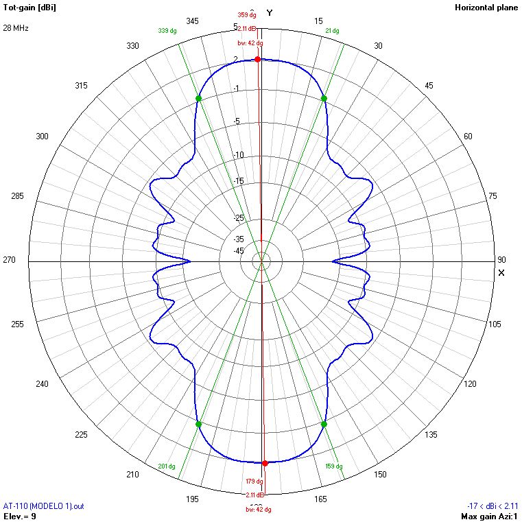
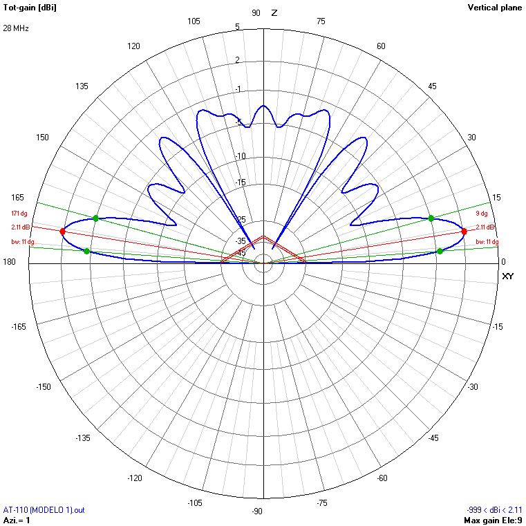
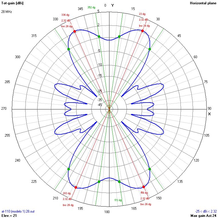
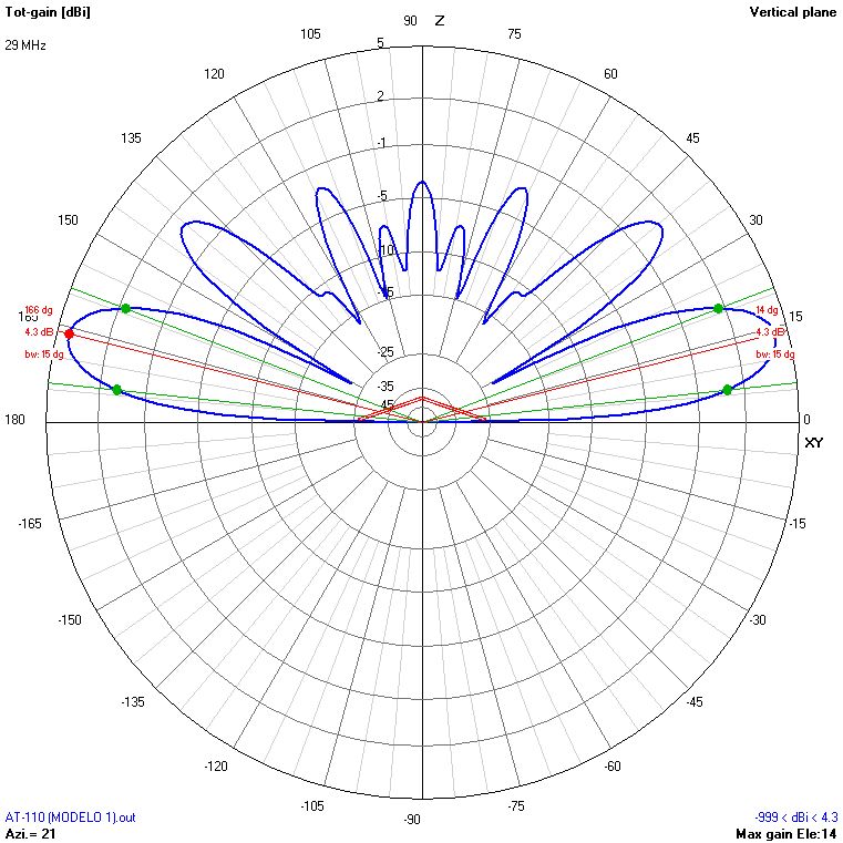
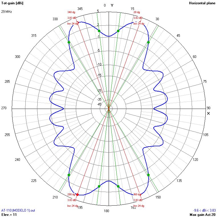
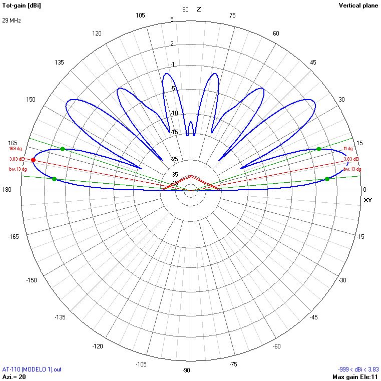
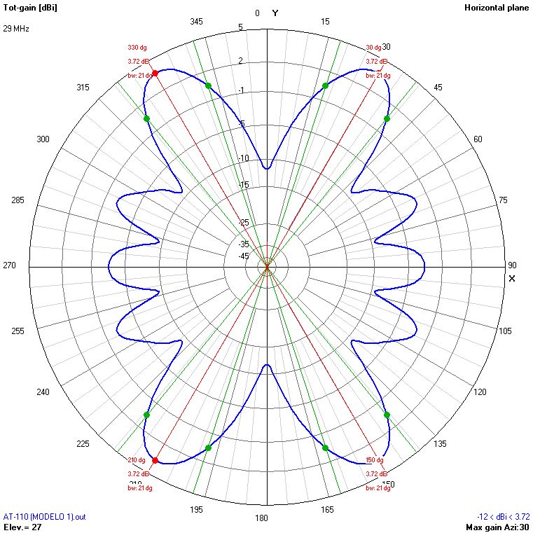
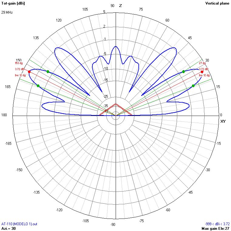
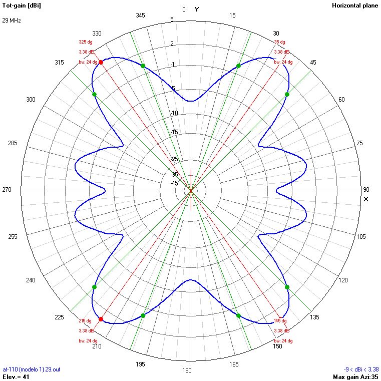
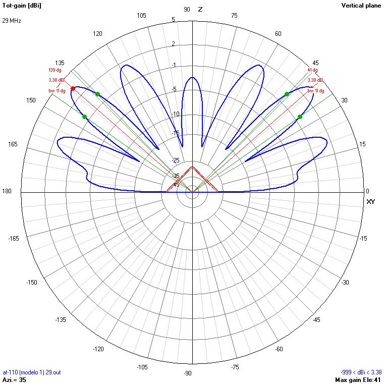
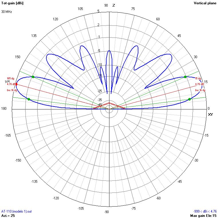
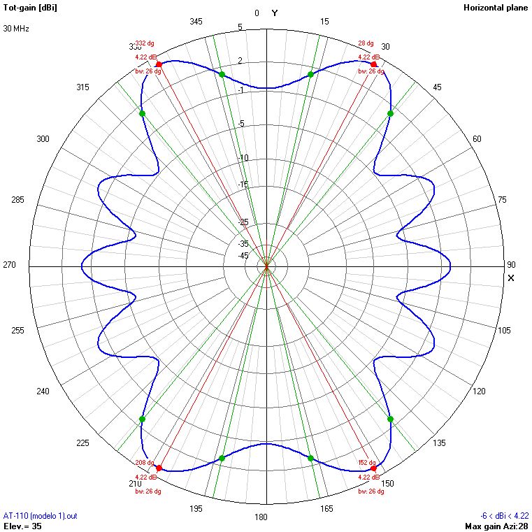
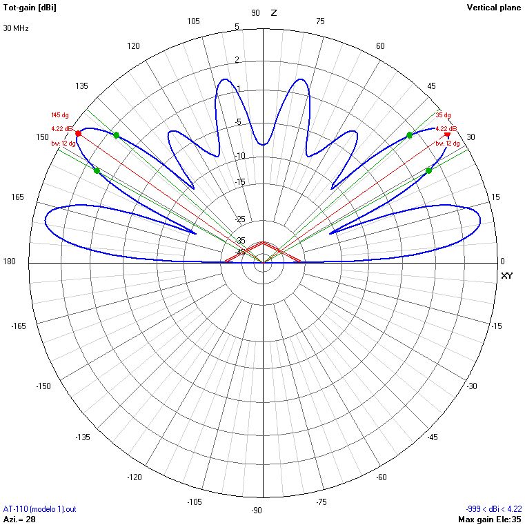
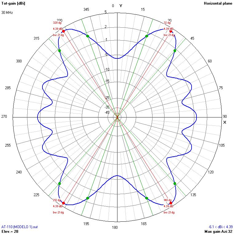
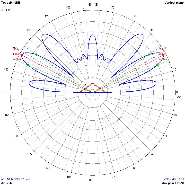
In this section, the results of the simulations of the model 1 are shown (see section 2.1), consisting on radiation patterns for frequencies between 2 MHz and 30 MHz at 1 MHz intervals and for masts of 9, 12, 15 and 18 m. The antenna is installed in inverted-vee configuration with the tips at 0,5 meters over ground.
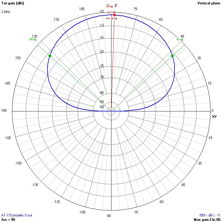
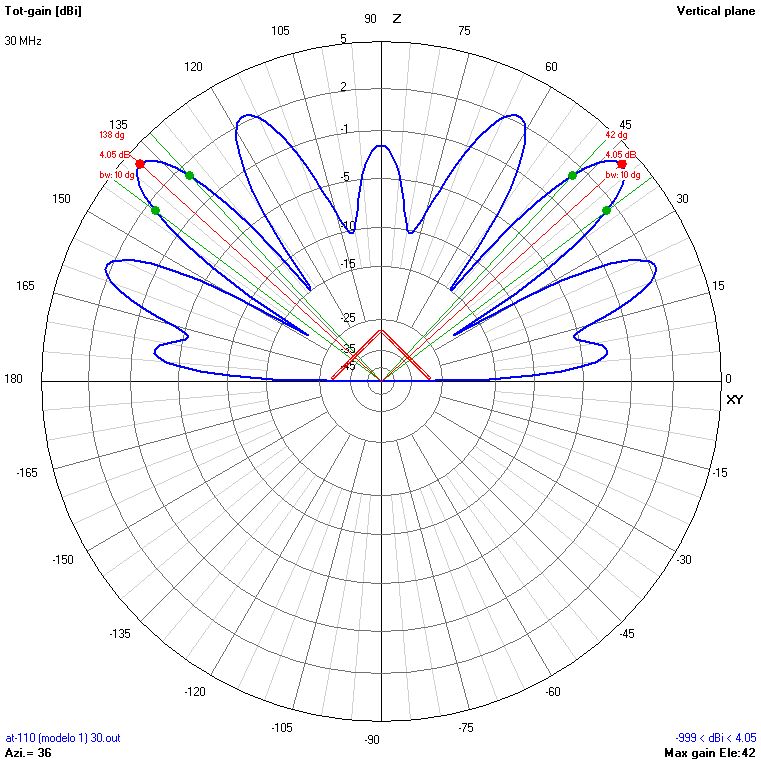
All the radiation patterns shown correspond to the planes of maximum radiation for each frequency. In the case of the vertical patterns, the angle of the azimuth plane where the cut has been made is shown. The same way, in the case of the horizontal patterns, the angle of the elevation plane where the cut has been made is shown. In all the cases, the antenna's position is sketched in red. Please take those considerations into account when comparing patterns of different frequencies.
Remember that in all the simulations, the azimuth is the horizontal angle with respect to the antenna (measured from the Y axis towards the X axis, clockwise). The elevation is the vertical angle with respect to the ground (measured from the Y axis towards the Z axis). The fig.2 shows a diagram explaining the reference system used.
This way, the antenna is always placed in the plane of azimuth 0º, being 90º the direction perpendicular to the antenna, towards the front. The 90º angle of elevation corresponds to the direction perpendicular to the ground (NVIS).
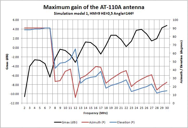
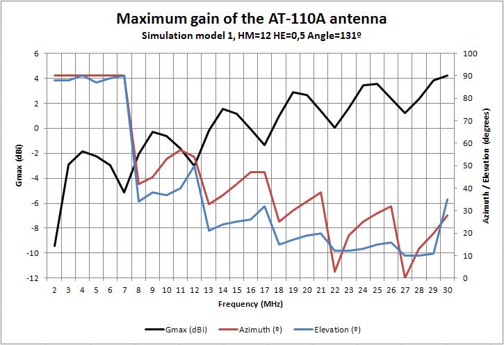
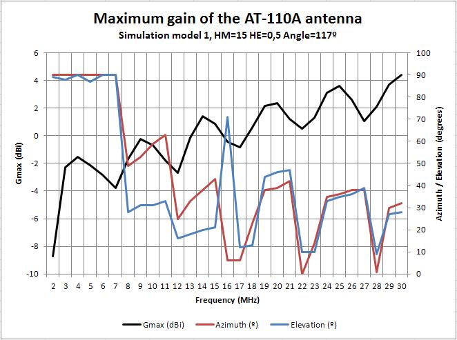
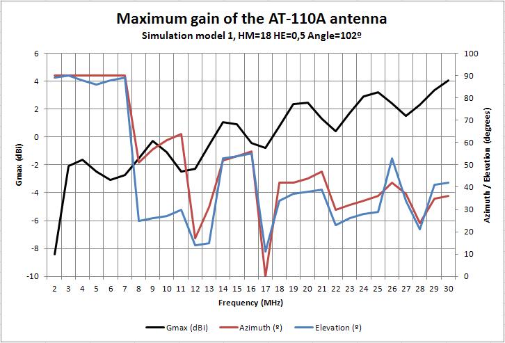
I will provide also a set of plots of maximum gain for each configuration of installation, indicating the values of azimuth and elevation where the maximum gain occurs. Those plots may be useful to point the antenna at the intended receiver on the other side of the radio link.
For each case, click on the image to see a larger version. The results will be discussed on the section 7.
The table 7 shows the radiation patterns corresponding to the installation of the antenna using masts of 9, 12, 15 and 18 meters.
| Frequency (MHz) | HM=9 Alpha=72,32º |
HM=12 Alpha=65,75º |
HM=15 Alpha=58,81º |
HM=18 Alpha=51,31º |
||||
|---|---|---|---|---|---|---|---|---|
| H | V | H | V | H | V | H | V | |
| 2 | 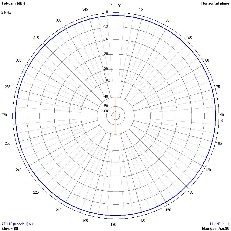 |
 |
 |
 |
 |
 |
 |
 |
| 3 | 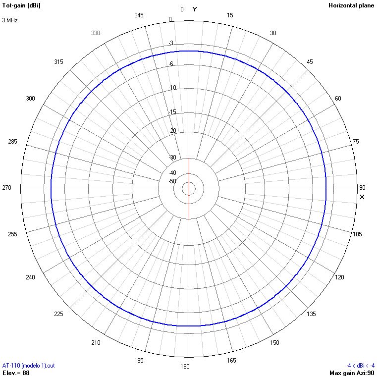 |
 |
 |
 |
 |
 |
 |
 |
| 4 | 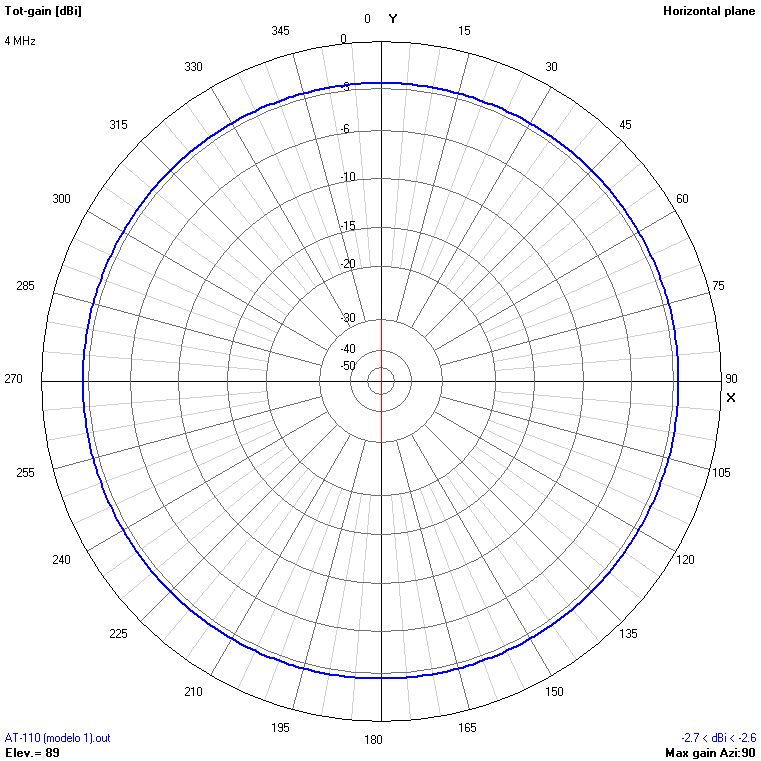 |
 |
 |
 |
 |
 |
 |
 |
| 5 | 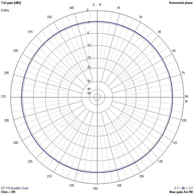 |
 |
 |
 |
 |
 |
 |
 |
| 6 | 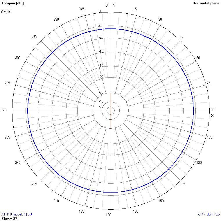 |
 |
 |
 |
 |
 |
 |
 |
| 7 | 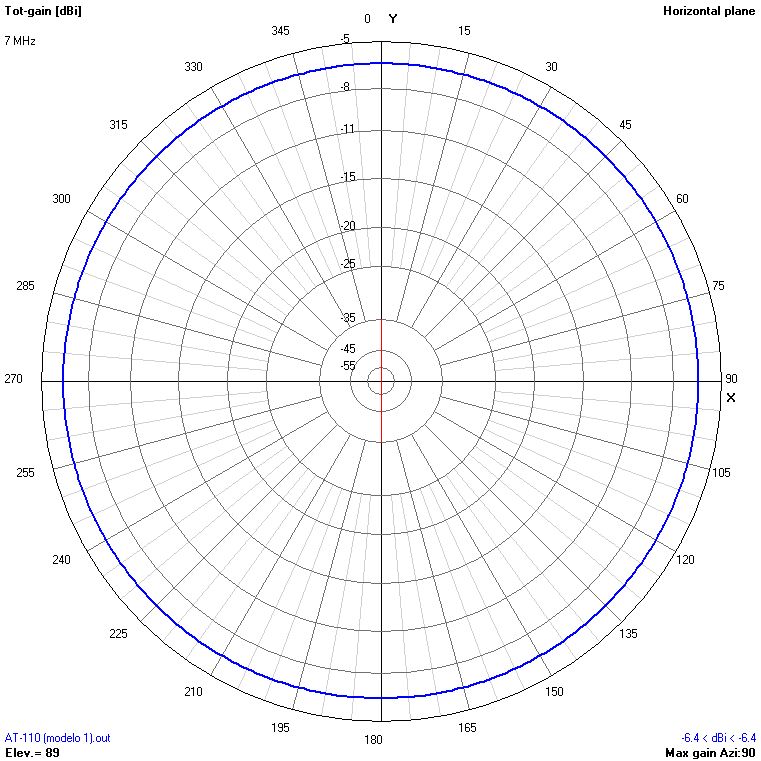 |
 |
 |
 |
 |
 |
 |
 |
| 8 | 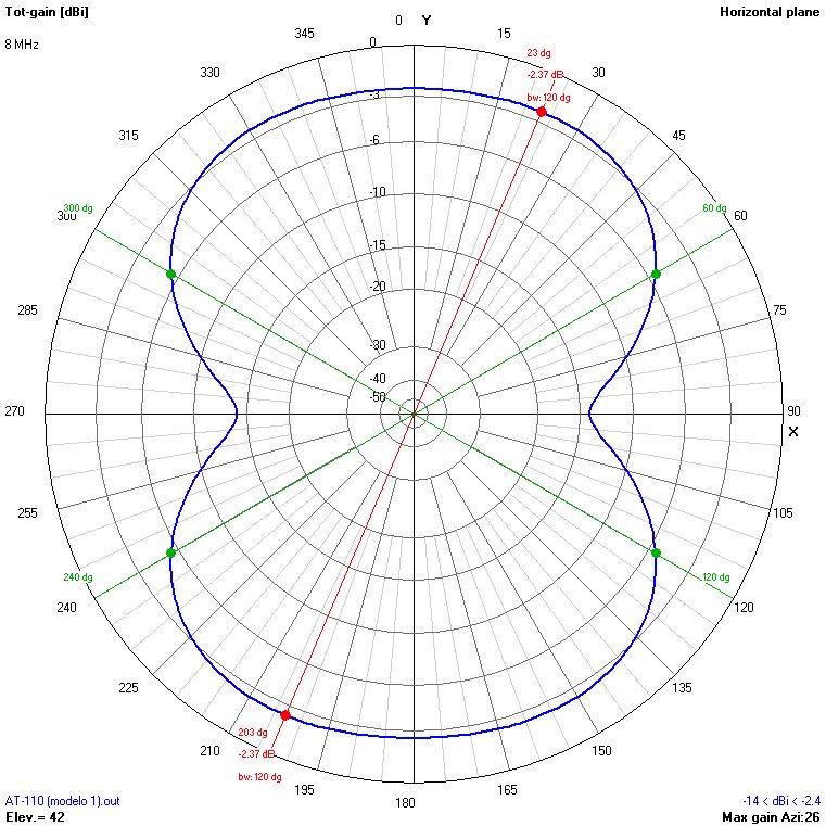 |
 |
 |
 |
 |
 |
 |
 |
| 9 | 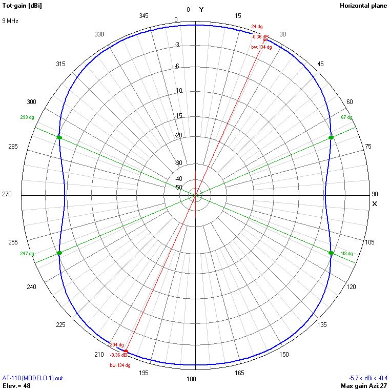 |
 |
 |
 |
 |
 |
 |
 |
| 10 | 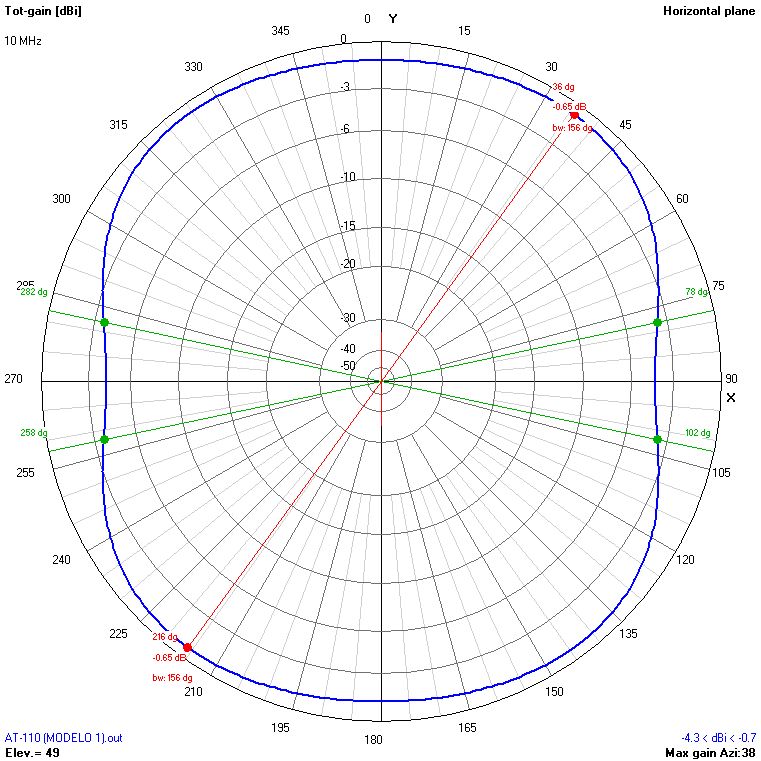 |
 |
 |
 |
 |
 |
 |
 |
| 11 | 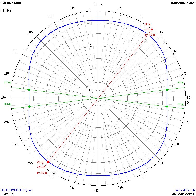 |
 |
 |
 |
 |
 |
 |
 |
| 12 | 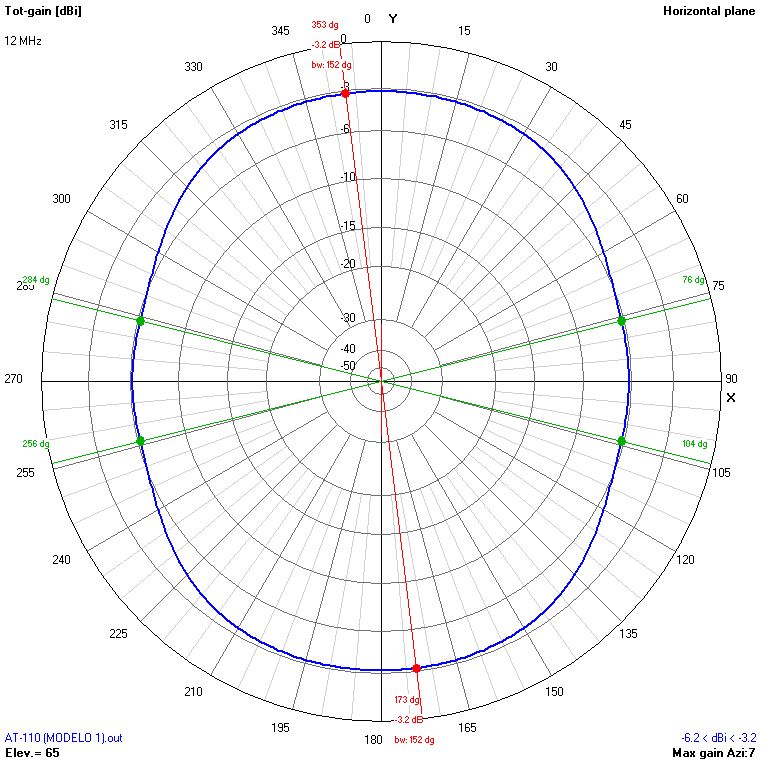 |
 |
 |
 |
 |
 |
 |
 |
| 13 | 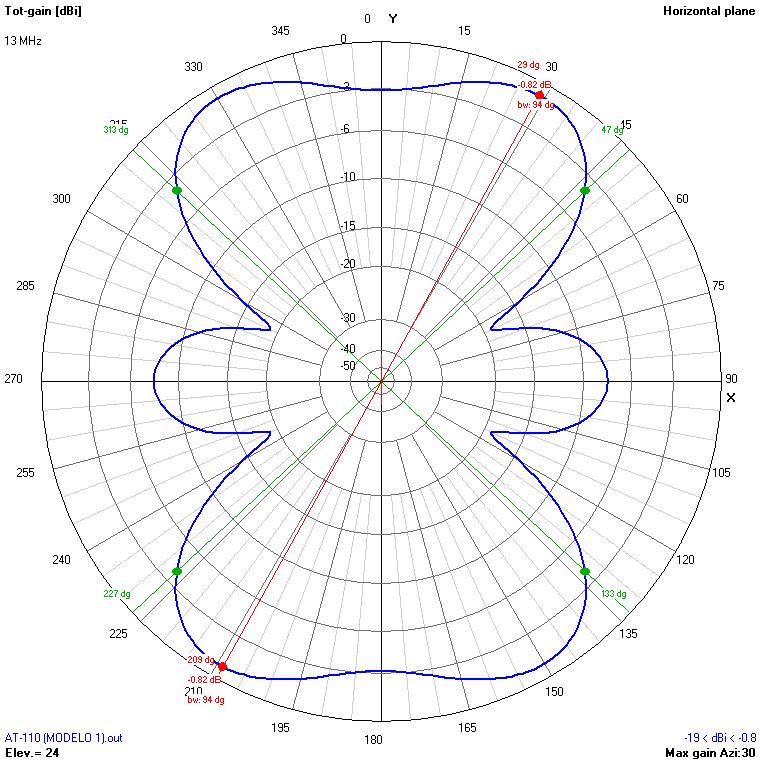 |
 |
 |
 |
 |
 |
 |
 |
| 14 | 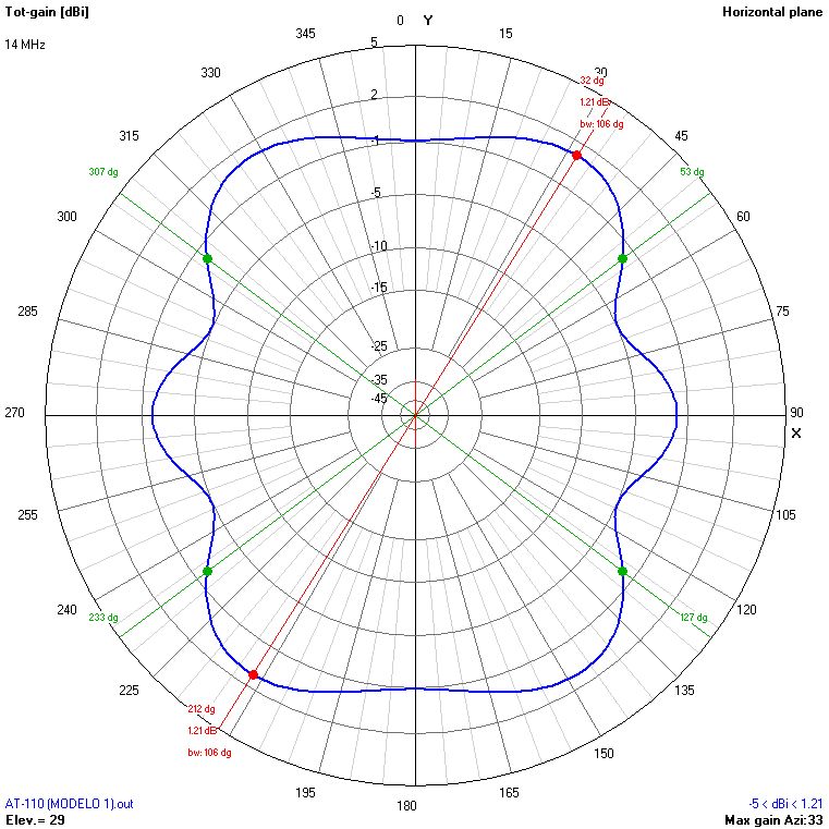 |
 |
 |
 |
 |
 |
 |
 |
| 15 | 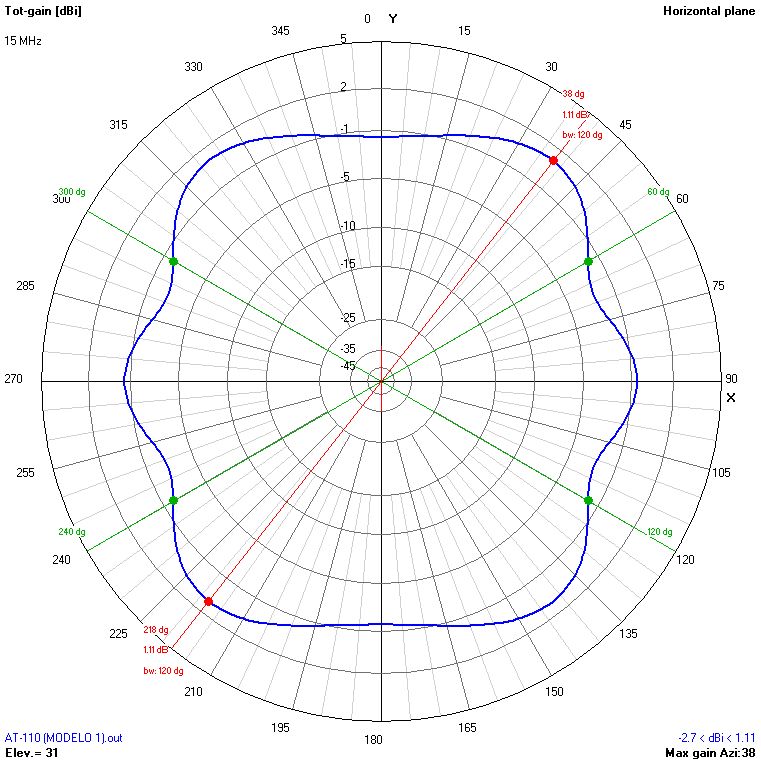 |
 |
 |
 |
 |
 |
 |
 |
| 16 | 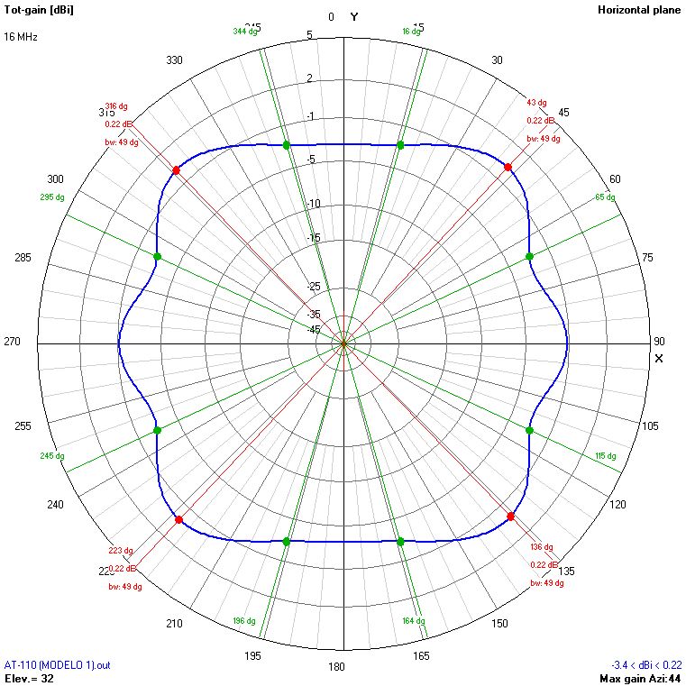 |
 |
 |
 |
 |
 |
 |
 |
| 17 | 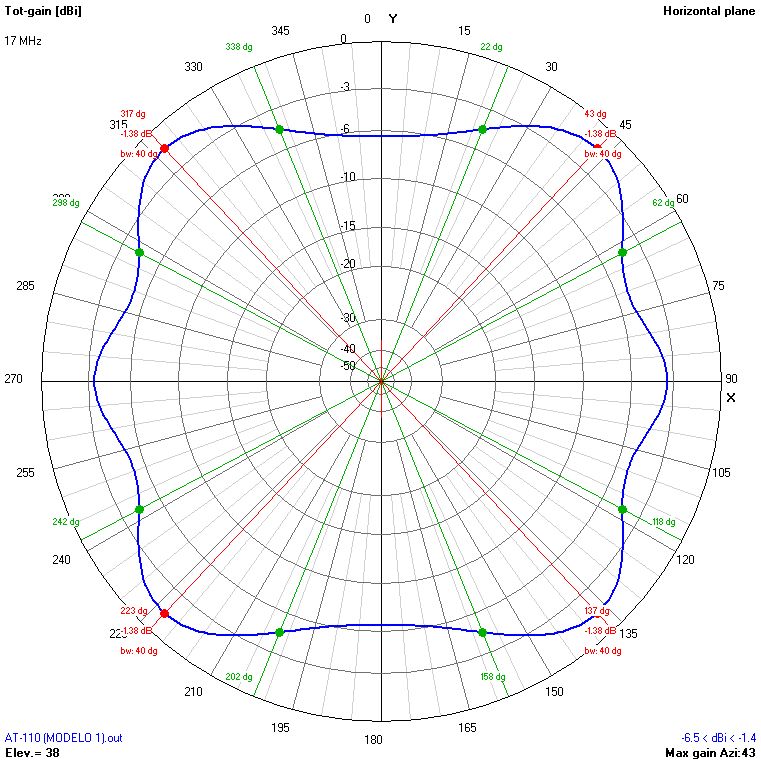 |
 |
 |
 |
 |
 |
 |
 |
| 18 | 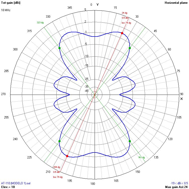 |
 |
 |
 |
 |
 |
 |
 |
| 19 | 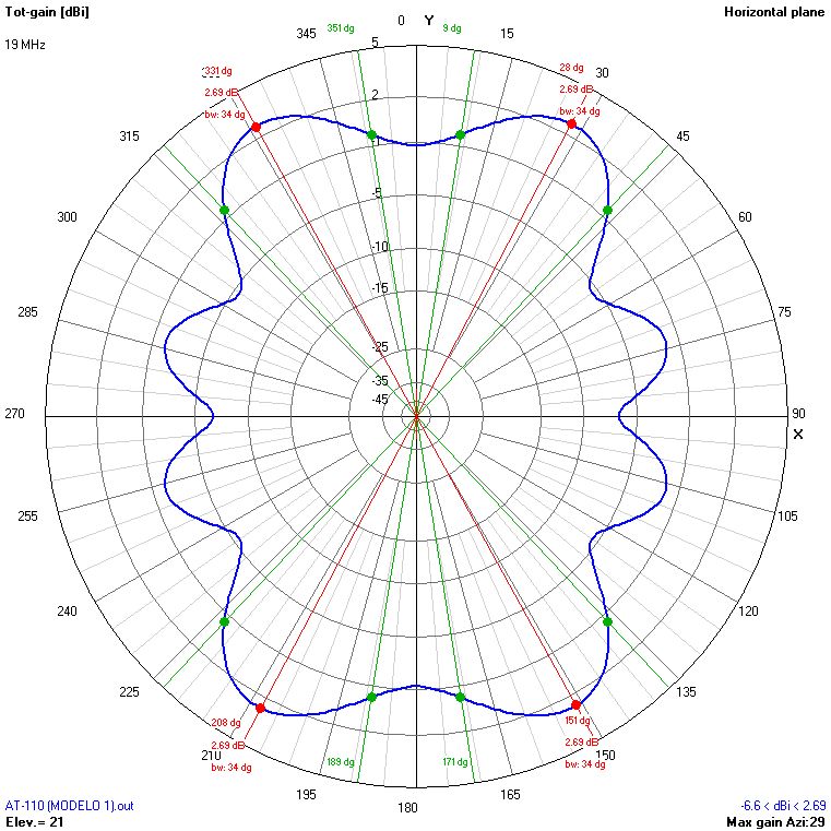 |
 |
 |
 |
 |
 |
 |
 |
| 20 |  |
 |
 |
 |
 |
 |
 |
 |
| 21 | 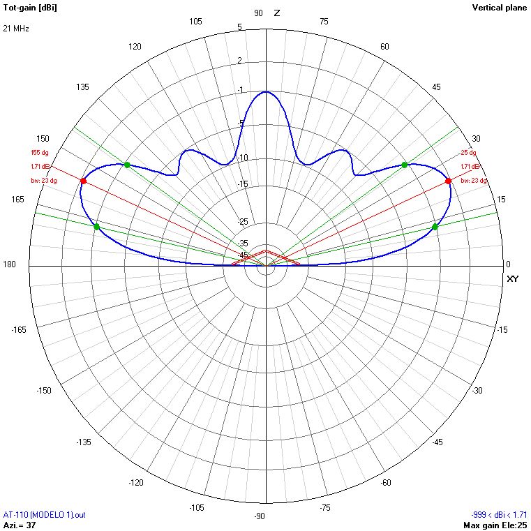 |
 |
 |
 |
 |
 |
 |
 |
| 22 | 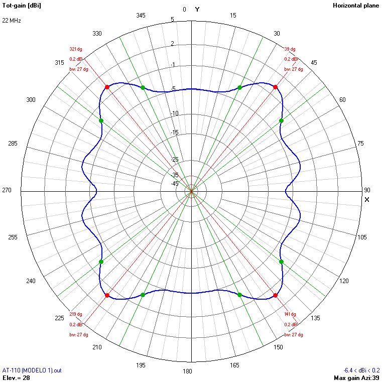 |
 |
 |
 |
 |
 |
 |
 |
| 23 | 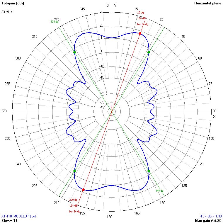 |
 |
 |
 |
 |
 |
 |
 |
| 24 | 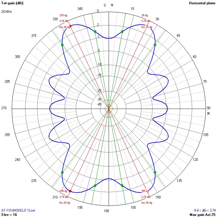 |
 |
 |
 |
 |
 |
 |
 |
| 25 | 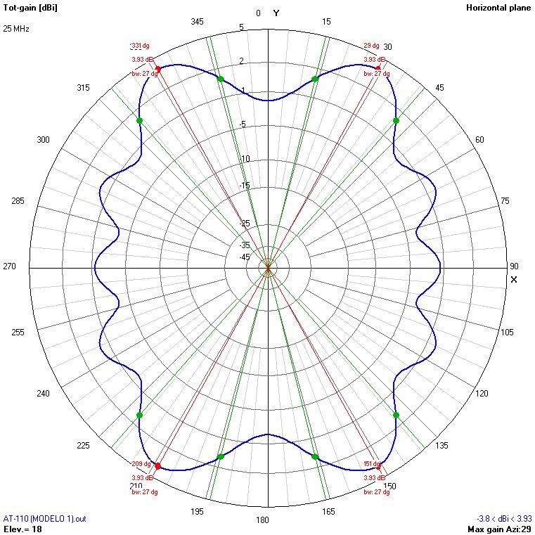 |
 |
 |
 |
 |
 |
 |
 |
| 26 | 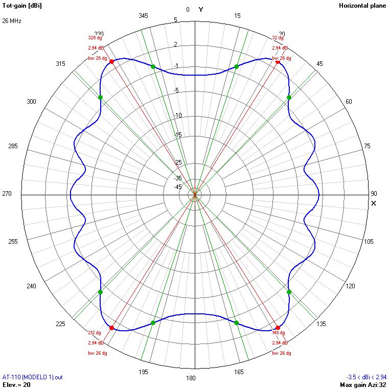 |
 |
 |
 |
 |
 |
 |
 |
| 27 | 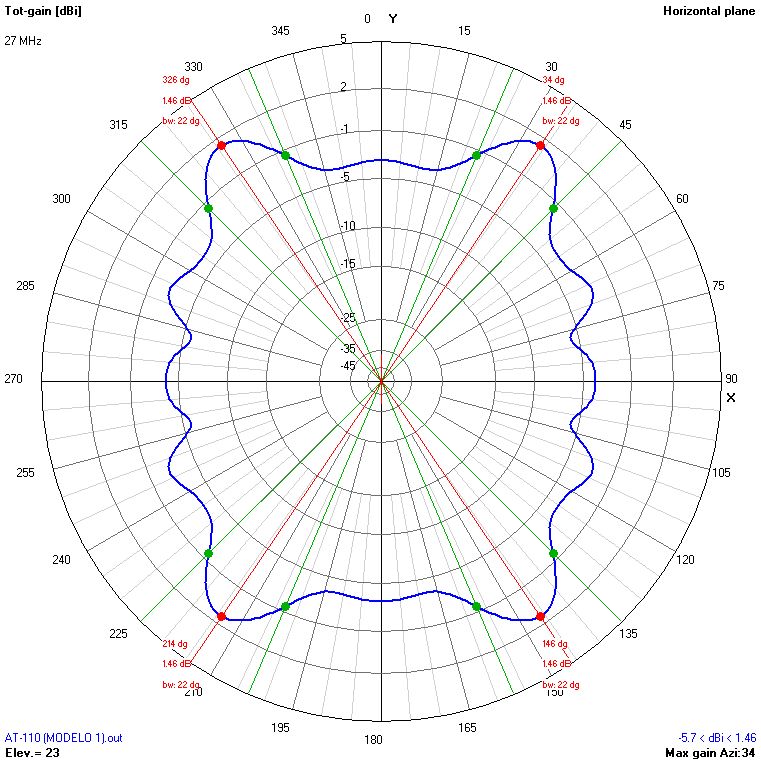 |
 |
 |
 |
 |
 |
 |
 |
| 28 | 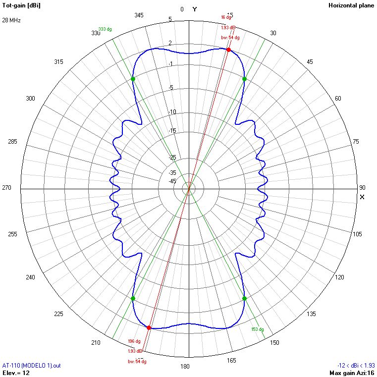 |
 |
 |
 |
 |
 |
 |
 |
| 29 | 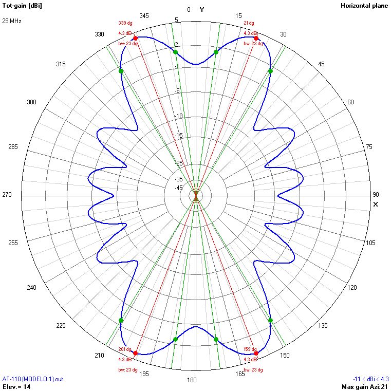 |
 |
 |
 |
 |
 |
 |
 |
| 30 | 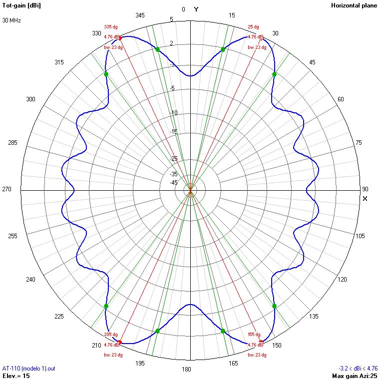 |
 |
 |
 |
 |
 |
 |
 |
Simulation model 1.
Below you will find the plots of maximum gain using masts of 9, 12, 15 and 18 meters. Click on each image to see a larger version.
The figure 6 shows the plot of maximum gain for a height of installation HM = 9 meters.
The figure 7 shows the plot of maximum gain for a height of installation HM = 12 meters.
The figure 8 shows the plot of maximum gain for a height of installation HM = 15 meters.
The figure 9 shows the plot of maximum gain for a height of installation HM = 18 meters.
Finally, the figure 10 shows a comparison of the maximum gain for the four installation configurations analysed.
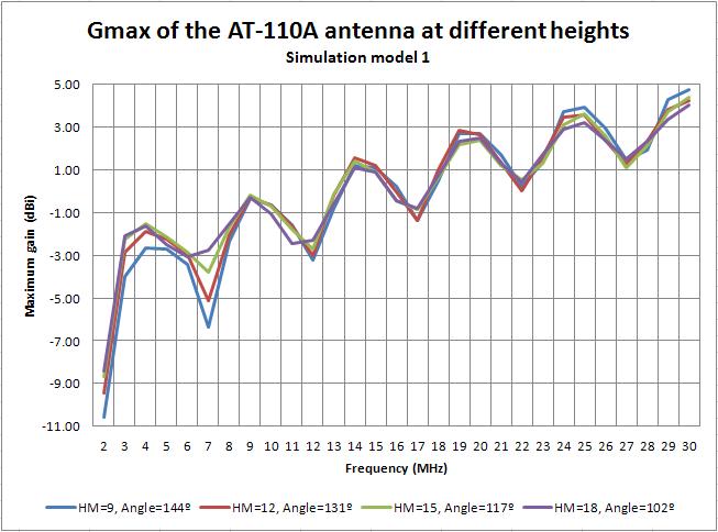
The results will be analysed on the section 7.


|
Ismael Pellejero - EA4FSI |
 EA4FSI Home |
 HF Antennas |
 HF Central |