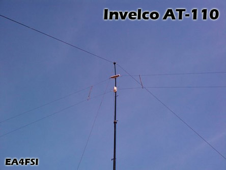
Invelco AT-110 folded dipole antenna

Main → HF Radio Resources Center → HF Antennas → Invelco AT-110 → Antenna modeling using 4Nec2

Este artículo también está disponible en Español (this article is also available in Spanish).

2. Antenna modeling using 4Nec2.

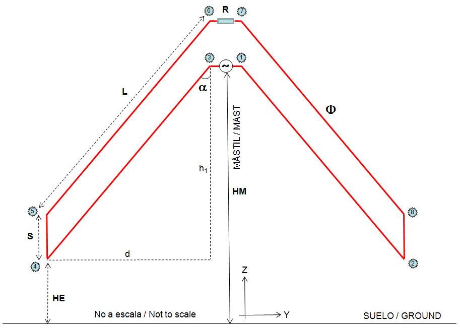
I have designed two different models of the Invelco AT-110 antenna in order to take into account several installation configurations. In both models, the following variables are considered:

F: working frequency (MHz).
L: antenna leg length (m).
S: distance between the two wires on each leg (m).
R: resistive load (ohms).
Phi: diameter of the antenna wire (mm).
HM: height of the mast when installing the antenna in inverted-vee configuration (m).
HE: height of the tips when installing the antenna in inverted-vee configuration (m).
Alpha: semi-angle formed by the two legs of the antenna (degrees).

The values of L, S, R and Phi are different for each model of the antenna (A/B/C) provided by the manufacturer and
can be checked in the user's manual.

The values of HM, HE and Alpha are related to the configuration used to install the antenna. Once the antenna is nstalled on top of a mast of height HM, it is possible to determine the height of the tips HE if the angle Alpha is known, or to calculate Alpha using the values of HM and HE.

The frequency band between Fmin = 2 MHz and Fmax = 30 MHz will be considered for all the simulations.

During the process of antenna modeling, I have taken into account the rules described in the "Notes on antenna
simulation using NEC-2", available in this web site.

The fig.2 shows the coordinate system used in the simulations. In the two sketches on the right part, the antenna
is represented in red. Click on the image to see a larger version:

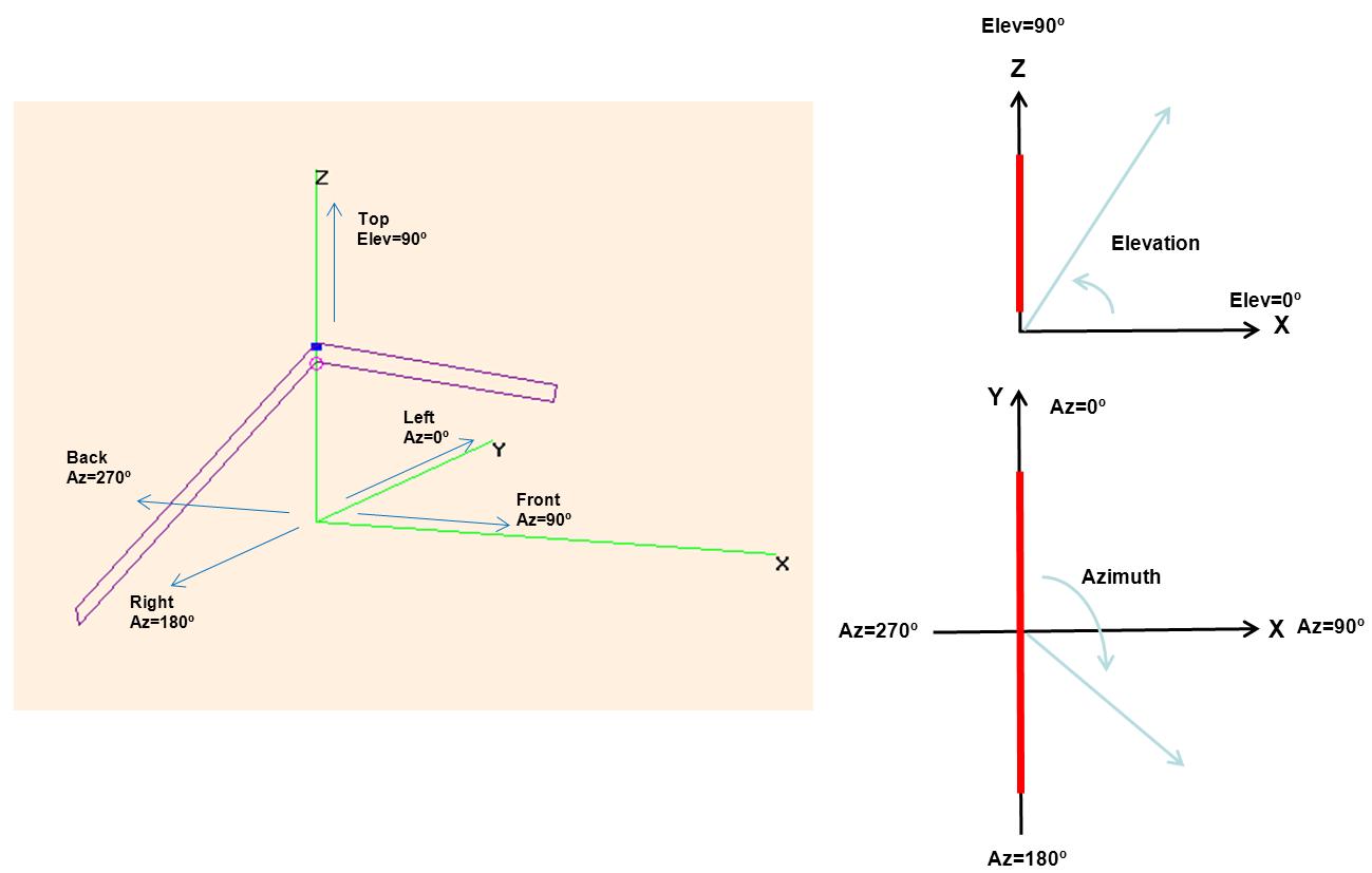
Fig.2. Conventions used in the simulations.

In this system, the following conventions are used:

The ground is defined by the XY plane.
The antenna is installed along the Y axis.
The height is measured along the Z axis.
The takeoff angle is measured from the ground (XY plane) towards the positive Z semi-axis, with possible
values between 0º (ground) and 90º (direction perpendicular to the ground).
The azimuth angle is measured from the positive Y semi-axis towards the positive X semi-axis, with possible
values between 0º and 360º. Thus, the different directions of interest are:

Azimuth = 0º: left side of the antenna.
Azimuth = 90º: front side of the antenna.
Azimuth = 180º: right side of the antenna.
Azimuth = 270º: back side of the antenna.

The mast of the antenna is not simulated in any case, so it is necessary to take into account that in a real installation it will affect both the impedance and the radiation patterns of the antenna with respect to the results of the simulations.

2.1. Model 1.

The fig.3 shows the first model used to simulate the antenna in 4Nec2. Click on the image to see a larger version.

Fig.3. Model 1.

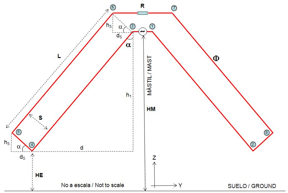
The wires of the model are numbered as shown in the table 1..

Wire	End 1	End 2
1	P1	P3
2	P3	P4
3	P4	P5
4	P5	P6
5	P6	P7
6	P7	P8
7	P8	P2
8	P2	P1

Table 1. Wires of the model 1.

In order to determine the coordinates of the 8 points delimiting each section of the model, we will use the following
trigonometric relations:

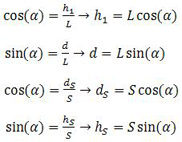
On the other and and as stated before, the height of installation of the tips of the antenna (HE) can be computed
using the height of the mast (HM) and the semi-angle formed by the legs of the antenna (Alpha). The same way, the angle Alpha can be computed using HM and HE, using the following formula. Remember that Alpha is half the angle formed by the two legs of the antenna. This way, an angle Alpha = 90º means that the antenna is installed horizontally.

In this model, an horizontal section of 0,5 m in length (wire 1) is used to install the generator, placed at a height
HM (height of the mast). This is the point of installation of the balun in the real antenna. This additional section
of the model is necessary to avoid having the generator on the tip of one of the wires, a configuration which may cause errors in the results obtained with the NEC-2 algorythm.

The antenna is deployed in inverted-vee configuration, being its tips at a height HE over the ground. On each leg, the sections of the antenna between the two main wires (wires 3 and 7, length S) are arranged perpendicular to them. Finally, the model includes another horizontal section of variable length on the top (wire 5) to place the resistive load. In this model I have considered that the two main wires of each leg have the same length L. Notice that using this model in inverted-vee configuration, the two horizontal wires (1 and 5) are separated a length slightly lower than S.

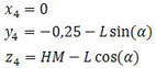
Using the draw and the trigonometric relations presented before, the coordinates of the 8 points of interest will be:

Coordinates of point 1:

Coordinates of point 2:

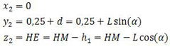
Coordinates of point 3:

Coordinates of point 4:

Coordinates of point 5:

Coordinates of point 6:

Coordinates of point 7:

Coordinates of point 8:

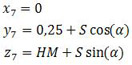
2.2. Model 2.

The fig.4 shows the second model used to simulate the antenna in 4Nec2. Click on the image to see a larger version.

Fig.4. Model 2.

The wires of the model are numbered as shown in the table 2.

Wire	End 1	End 2
1	P1	P3
2	P3	P4
3	P4	P5
4	P5	P6
5	P6	P7
6	P7	P8
7	P8	P2
8	P2	P1

Table 2. Wires of the model 2.

The antenna is deployed in inverted-vee configuration, being its tips at a height HE over the ground. On each leg, the sections of the antenna between the two main wires (wires 3 and 7, length S) are arranged perpendicular to the ground. Finally, the model includes another horizontal section of variable length on the top (wire 5) to place the resistive load. In this model I have considered that the two main wires of each leg (wires 2-4 and 6-8) have the same length L.

In this case and in contrast to the first model, the two horizontal wires (1 and 5) are always separated a length S.

In order to compute the coordinates of the points of interest, we can use the same trigonometric relations shown in the section 2.1.

Coordinates of point 1:

Coordinates of point 2:

Coordinates of point 3:

Coordinates of point 4:

Coordinates of point 5:

Coordinates of point 6:

Coordinates of point 7:

Coordinates of point 8:

Using this model it is necessary to take into account that, if using autosegmentation in 4Nec2, there will be parallel wires with different number of segments, a fact which may have some influence on the results of the simulations.