EA4FSI — Geometry and operative aspects of the simple modes of ionospheric propagation

Ionospheric propagation of radio waves involves complex mechanisms such as refraction and diffraction, which depend, among other factors, on the degree of ionisation and the frequency used. This article uses a simplified model based on pure ionospheric reflections, solely to provide an approximation for calculating hop distances and coverage areas.

1. Analysis for one hop.

In order to analyse the geometry of an ionospheric radio link, we can study the geometry for only one hop and extrapolate the results. We will use the diagram shown in Figure 1.

Fig.1. Geometry of one ionospheric hop

The following parameters are known:

The location of the radio transmitter on the Earth's surface.
The antenna take-off angle. When the antenna points towards the horizon, this angle is zero.
The altitude of the layer of the ionosphere where reflection occurs.
The radius of the Earth (6370 km).

Ionospheric reflections will normally occur at altitudes of approximately 100 km (E layer or sporadic E layer) or 300 km (F layer).

The radio links using only one of the layers as a reflector follow the simple propagation modes, which are named with a number indicating the number of hops, and a letter identifying the layer of the ionosphere used. This way, the mode of propagation using one hop in the F layer is called 1F mode, 2F for two hops and so on. In a general way, we call those modes "nF", for "n" hops.

The same applies in the case of reflections in the E layer: for "n" hops, we will use the "nE" notation.

2. Length of the radio path.

Determining the length of the radio path will serve to compute the propagation losses and the distance reached by every hop.

In each hop, the radio wave will travel twice the distance "d": once between the transmitter "TX" and the point "I" in the ionosphere, and once between this point and the point "P" located at the Earth's surface.

In order to compute "d", we will use the triangle formed by the points "TX-I-C" and the law of cosines:

{R_{T} + H}^{2} = d^{2} + {R_{T}}^{2} + 2 d R_{T} \cos (90 + β)

[1]

If we evaluate the term on the left side of [1], we obtain the following quadratic equation [2], being "d" the unknown:

d^{2} + 2 d R_{T} \cos (90 + β) - H (H + 2 R_{T}) = 0

[2]

The solution of this equation is [3]:

d = \frac{- 2 R_{T} \cos (90 + β) \pm \sqrt{{(2 R_{T} \cos (90 + β))}^{2} + 4 H (H + 2 R_{T})}}{2}

[3]

That is, we can compute the distance "d" using the radius of the Earth, the antenna's take-off angle and the altitude of the point where ionospheric reflection occurs.

3. Hop distance.

The hop distance is two times the arc length between the points "TX" and "P". The arc length can be computed using the formula [4]:

d_{A} = \frac{2 π R_{T} α}{360}

[4]

To compute this distance, it is necessary to know the value of the angle alpha (in degrees). We can compute alpha first using the law of sines for the triangle "TX-I-C":

\frac{R_{T} + H}{\sin (90 + β)} = \frac{R_{T}}{\sin (γ)} = \frac{d}{\sin (α)}

[5]

Now, using the first and last terms of [5]:

\sin (α) = \frac{d \sin (90 + β)}{R_{T} + H} ⟹ α = \arcsin [\frac{d \sin (90 + β)}{R_{T} + H}]

[6]

Where the distance "d" between the points "TX" and "I" was calculated using [3].

Therefore, if we use [4] and [6], the resulting hop distance is [7]:

d_{HOP} = 2 d_{A} = \frac{4 π R_{T} \arcsin [\frac{d \sin (90 + β)}{R_{T} + H}]}{360}

[7]

That is, the hop distance can be computed using the radius of the Earth, the antenna's take-off angle, the altitude of the point where ionospheric reflection occurs and the distance from the transmitter to this point in the ionosphere.

4. Coverage areas.

Having established the method for calculating hop distances, it is easy to calculate the coverage areas of the transmitter using a particular take-off angle and one layer of the ionosphere as a reflector.

In this section, the analysis provided will be solely geometrical and it will be necessary to take into account the power budget in order to check whether the radio links are possible for each coverage area computed.

In each hop, the maximum distance is reached using a take-off angle of zero degrees, that is, with the antennas pointing to the horizon, using a radio path tangent to the Earth's surface.

However, the radiation pattern of a directional antenna has a −3 dB beamwidth which we need to take into account, so it is common to suppose that under those circumstances the antenna radiates with take-off angles between 0 degrees and 2 degrees.

The wave taking off at 2 degrees will be reflected in the ionosphere with an angle of incidence higher than the angle of the wave taking off at 0 degrees, so it will be reflected again in the Earth's surface at a lower distance than those of the latter. We will study those two rays demarcating the radiation of the antenna. The ray taking off at 0 degrees provides the maximum range and the ray taking at 2 degrees provides the minimum range at each hop. Those ranges can be computed using [7].

Also, using [4], we can compute the distances from the transmitter where reflection at the ionosphere occurs.

In Figure 2, the wave taking off at 0 degrees is represented by the blue ray and the wave taking off at 2 degrees is represented by the red ray, using a flat model both for the Earth's surface and the ionosphere. The scale has been exaggerated for better interpretation.

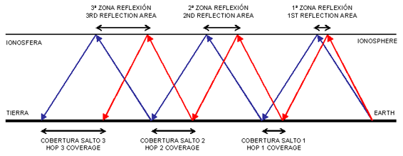
Fig.2. Coverage areas of successive hops

As we can see in Figure 2, the effect caused by the different angles of incidence makes the consecutive coverage areas wider, as the wavefront advances.

If we suppose that reflection occurs in the E layer or the sporadic E layer of the ionosphere, at an altitude of 100 km, we will have the coverage areas shown in the table 1.

Hop	Minimum range (km)	Maximum range (km)
1	1841	2243
2	3683	4486
3	5524	6728
4	7365	8971
5	9207	11214

Table 1. Coverage areas of nE modes

For those same nE modes, the table 2 shows the areas where reflection at the ionosphere occurs.

Hop	Minimum range (km)	Maximum range (km)
1	921	1121
2	2762	3364
3	4603	5607
4	6445	7850
5	8286	10093

Table 2. Areas of reflection in the ionosphere for the nE modes

If we suppose now that reflection occurs in the F layer of the ionosphere, at an altitude of 300 km, we will have the coverage areas shown in the table 3.

Hop	Minimum range (km)	Maximum range (km)
1	3416	3836
2	6831	7671
3	10247	11507
4	13663	15342
5	17079	19178

Table 3. Coverage areas of nF modes

For those same nF modes, the table 4 shows the areas where reflection at the ionosphere occurs.

Hop	Minimum range (km)	Maximum range (km)
1	1708	1918
2	5124	5753
3	8539	9589
4	11955	13424
5	15371	17260

Table 4. Areas of reflection in the ionosphere for the nF modes

In this case, due to the fact that the altitude where the ionospheric reflection occurs is higher, each hop in the nF modes is larger than the hops in the nE modes. An additional advantage of the nF modes is that, for a given distance, the radio wave travels less time through the absorptive D layer of the ionosphere.

In all cases described, the computed distances may be different as a function of the exact altitude of the point where ionospheric reflection occurs, so the values shown are intended as approximate estimates.

The computed data can be represented in geographical information systems and applications, such as Google Earth, which will allow to check easily the areas of coverage for each mode. The fig.3 shows an example of the approximate coverage of the nE modes from the Canary Islands (EA8).

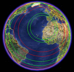
Fig.3. Coverage areas of nE modes from the Canary Islands

5. Power budget.

The power budget is the result of computing the transmission equation for a given radio link. We will use the sketch shown in Figure 4 as a reference.

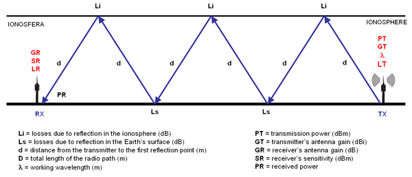
Fig.4. Parameters of the transmission equation

The transmission equation is given by [8]:

P_{R} = \frac{P_{T} G_{T} G_{R}}{L {(\frac{4 π D}{λ})}^{2}} \geq S_{R}

[8]

That is, at the receiver's side, the received power must be higher than the receiver's sensitivity in order for the radio link to work.

Transmitter power and antenna gain contribute positively to the link budget.

On the other hand, several parameters weigh against the power budget: the free space transmission loss (the quadratic term between parenthesis in the denominator), the transmission lines and connector losses, the reflection losses in the ionosphere ("Li") and the reflection losses in the Earth's surface ("Ls"). All the referred losses but the free space ones are grouped in the term "L" in [8].

The losses due to reflections in the ionosphere and in the Earth's surface are quite difficult to estimate because they depend on several factors, such as the density of ionization of the ionospheric layers or the electrical conductivity of the surface of the Earth. I.e., if the wave is reflected from the sea surface the losses will be much lower than in the case of a reflection in the land.

We can make a coarse approach of those losses, considering that in each ionospheric reflection we have an attenuation "Li" of 5 dB in the first hop, 5 dB in the second hop, 3,5 dB in the third hop and 2,5 dB for each consecutive hop. In the case of the reflections in the Earth's surface, we will use additional losses "Ls" of 3,5 dB for each hop.

The distance "D" in [8] is the total length of the radio path, being equal to the sum of all paths of length "d" shown in Figure 4, whose value can be computed using [3].

The transmission equation [8] can be expressed in logarithms, resulting [9]:

P_{R} (dBm) = P_{T} (dBm) + G_{T} (dB) + G_{R} (dB) - L (dB) - 20 \log (\frac{4 π D}{λ})

[9]

Once computed the received power and being known the receiver's sensitivity, the fading margin is defined as [10]:

MF (dB) = P_{R} (dBm) - S_{R} (dBm)

[10]

If the fading margin is positive, the radio link can be established and its value is the amount of extra dB available to face other events causing attenuation, such as multipath propagation or geomagnetic storms. If the fading margin is negative, the signal level is below the sensitivity threshold of the receiver and cannot be demodulated.

Let's see an example of ionospheric radio link with the following characteristics:

Working frequency in the 7 MHz band (40 meters).
Transmission power: 100 W (50 dBm).
Antennas pointing to the horizon with a gain of 7 dB both in the transmitter and the receiver.
Receiver sensitivity: -123 dBm.
Transmission line losses of 1 dB both in the transmitter and the receiver.

We will analyse the available fading margins for the different nE and nF modes.

For each mode, we will compute the total length of the radio path ("D"), using the formula [3]. We will consider that the reflections in the E layer occur at an altitude of 100 km and the reflections in the F layer occur at an altitude of 300 km.

Considering the number of hops in each mode and using the theoretical values of "Li" and "Ls" stated before, we can compute the total attenuation "L" of the radio circuit. Using [9] we can compute the receiver power and then the fading margin using [10].

The results for the nE modes are shown in the table 5.

Mode	Length of radio path (km)	Received power (dBm)	Fading margin (dB)
1E	2266	-64	58
2E	4533	-73	49
3E	6799	-84	38
4E	9065	-92	30
5E	11331	-100	22

Table 5. Power budgets for the nE modes

The results for the nF modes are shown in the table 6.

Mode	Length of radio path (km)	Received power (dBm)	Fading margin (dB)
1F	3956	-69	53
2F	7912	-78	44
3F	11867	-89	33
4F	15823	-97	25
5F	19779	-105	17

Table 6. Power budgets for the nF modes

As stated before, these values are intended as approximate estimates due to the reasons exposed.

6. Maximum usable frequency.

The URSI defines the maximum usable frequency (MUF) as "the maximum frequency for ionospheric transmission using an oblique path, for a particular given system".

The MUF depends on several factors such as the altitude of the point where the ionospheric reflection occurs, the density of ionization in this point and the angle of incidence of the radio wave in the ionosphere.

In practice, we can compute the MUF using the data provided by the ionospheric sounding stations, also known as ionosondes. Those instruments measure several parameters of the ionosphere, such as the altitude and thickness of each layer and their critical frequencies. All those data gathered is represented in ionograms.

The critical frequency (fo) is the maximum frequency of a radio wave transmitted to the ionosphere with an angle of incidence of 90 degrees , that is, using a path perpendicular to the ionosphere from the Earth's surface. Each layer of the ionosphere has its own critical frequency, which changes with the hour of the day: foE for the E layer, foEs for the sporadic E layer, foF2 for the F2 layer, etc.

In Spain, there are two ionospheric sounding stations providing data to the public:

Ionograms from both ionosondes can be viewed in real time in the HF and Space Weather Panel.

The figure 5 shows an ionogram from the Ebro Observatory, generated the 04/22/2010 at 16:30 UTC. In the upper left side we can see that the critical frequency of the F2 layer was foF2 = 6.525 at this definite hour.

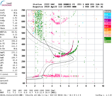
Fig.5. Ionogram from the Ebro Observatory generated on 04/22/2010 at 16:30 UTC

Knowing the fo of a layer of the ionosphere and using again the sketch of fig.1, we can compute the MUF as follows [11]:

MUF = \frac{f_{o}}{\sin (90 - γ)}

[11]

That is, for a given layer of the ionosphere, the maximum usable frequency is the quotient between the critical frequency and the sine of the angle of incidence of the radio wave in this layer.

In order to calculate the angle of incidence in the ionosphere, whose sine is in the denominator of [11], we consider that the take-off angle of the antenna is known and we calculate the angle alpha using [6]. Then, we consider that the sum of all the angles in a triangle is 180º, resulting [12]:

γ = 180 - α - (90 + β) = 90 - α - β

[12]

Using this angle and the fo value measured by the ionosonde, we can compute the MUF for circuits where the ionospheric reflection point is near the ionosonde. For multiple reflections, we may expect that for every point of reflection in the ionosphere the fo will be different for several reasons, i.e. the circuit may go through different areas of day and night where the density of ionization is different. In this case, we will calculate the MUF at each point of reflection in the ionosphere, being the resulting MUF of the circuit the minimum of them.

Analysing the data provided by an ionosonde, specifically the values of the critical frequencies of each layer, we may wonder whether those values are high enough to allow working in a particular band. For example, suppose an ionosonde has detected a sporadic E layer and is providing its measured critical frequency, foEs. Will this foES be high enough to allow working, i.e. in the 50 MHz band?

To answer that question, if we fix a minimum MUF for each band in [11], let's say 50 MHz, 144 MHz or 430 MHz, and using [12] we compute the angle of incidence in the ionosphere at every possible altitude of the point of reflection in the ionosphere, we will obtain the following graphs. We still suppose that the antennas are pointing to the horizon, so for each altitude the point of reflection in the ionosphere will be at increasing distances from the transmitter.

The graph in the fig.6 shows the minimum fo necessary to have a MUF allowing to work in the 50 MHz band (6 m).

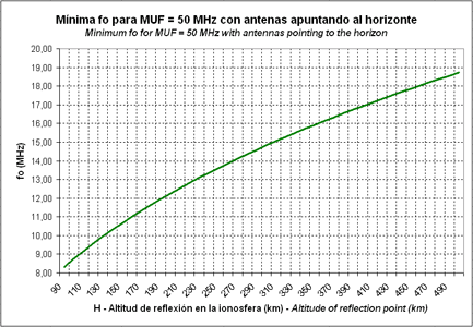
Fig.6. Minimum fo necessary to have a MUF allowing to work in the 50 MHz band

The graph in the fig.7 shows the minimum fo necessary to have a MUF allowing to work in the 144 MHz band (2 m).

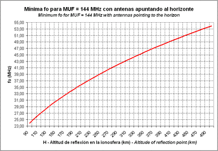
Fig.7. Minimum fo necessary to have a MUF allowing to work in the 144 MHz band

And finally, the graph in the Figure 8 shows the minimum fo necessary to have a MUF allowing to work in the 430 MHz band (70 m).

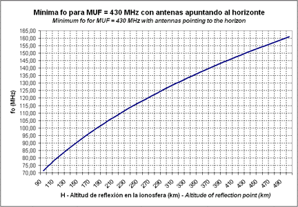
Fig.8. Minimum fo necessary to have a MUF allowing to work in the 430 MHz band

For instance, we want to know the minimum critical frequency of a sporadic E layer, measured by an ionosonde, which will allow to work in 50 MHz. If the sporadic E layer is located at an altitude of 100 km, checking the graph of the fig.6 we see that the minimum foEs must be of 8.75 MHz. If we want to work this sporadic layer in 144 MHz, the minimum foEs must be of 25,22 MHz (fig.7) and in order to work in 430 MHz the foEs must be of 75,31 MHz (Figure 8).

On 22 April 2010, several contacts between EA and DL-SP-OK were registered in the 50 MHz band, between 16:30-17:30 UTC. If we see again the ionogram shown in the fig.5, which was generated at the same hour, we can see that there was a sporadic E layer whose critical frequency was foEs = 7,60 MHz. Although it didn't reach the minimum theoretical value of 8.75 MHz, it was a good indicator of a sporadic E layer which at some distance from the ionosonde (at a point where foES > 8.75 MHz) allowed working at 50 MHz. The data provided by the ionosondes can serve as a good indicator of openings of propagation in each band.

7. Conclusions.

In the simple modes of ionospheric propagation, the same layer of the ionosphere is used as a reflector to establish the radio links, being usually the E layer, the sporadic E layer or the F layer. Each mode is defined by the geometry of the link, the power budget and the maximum usable frequency.

The study of the geometry of the link allows to compute in which zones of the ionosphere reflection occurs, and also in which areas of the Earth's surface coverage of the transmitter will exist. Both ranges can be calculated using the antenna take-off angles, the radius of the Earth and the altitude of the point of reflection.

In order to compute the power budget, we need to take into account the total length of the radio path, the working frequency, the transmission power, the transmission line losses and the receiver's sensitivity. The losses inherent to the ionospheric propagation, due to absorption and reflections, are difficult to estimate but may be approached by theoretical values. The resulting power budget will provide the available fading margin of the radio link.

To conclude, the maximum usable frequency can be computed with the help of the ionograms provided by ionospheric sounding stations, knowing the critical frequencies of each layer of the ionosphere and the angle of incidence of the radio waves. Surveillance of real time ionograms is a good method to watch openings in each band. Graphs to help to detect openings in 50 MHz, 144 MHz and 430 MHz are provided in this article.