 EA4FSI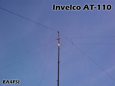
1. Introduction.
The AT-110 antenna is delivered in three different models (A/B/C), a resistively loaded folded dipole designed for broadband operation in the HF and part of the MF bands. It is a design of the Spanish company "Investigaciones Electrónicas y Comunicaciones (INVELCO)":
According to the manufacturer, the AT-110 family is designed to work in the frequency range between 1.5 MHz and 30 MHz, with a maximum power of 150 W or 1.5 kW (depending on the version) and radiation patterns similar to the presented by an inverted-vee dipole. Fig. 1 shows an AT-110A antenna mounted in inverted-vee configuration.
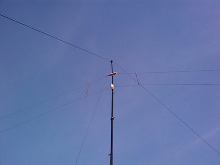
Fig. 1. Invelco AT-110 antenna.
The following sections provide the details of the simulations made with 4NEC2 (based on the NEC-2 algorithm) and using two different models with the goal of computing the standing wave ratio (SWR) and the radiation patterns of the antenna in all the working band.
2. Antenna modelling using 4NEC2.
Two different models of the Invelco AT-110 antenna have been developed in order to take into account several installation configurations. In both models, the following variables are considered:
-
F: working frequency (MHz).
-
L: antenna arm length (m).
-
S: distance between the two wires on each arm (m).
-
R: resistive load (ohms).
-
φ: diametre of the antenna wire (mm).
-
HM: height of the mast when installing the antenna in inverted-vee configuration (m).
-
HE: height of the antenna ends when installing the antenna in inverted-vee configuration (m).
-
α: semi-angle formed by the two legs of the antenna (degrees).
The values of L, S, R and φ are different for each model of the antenna (A/B/C) provided by the manufacturer and can be checked in the user's manual.
The values of HM, HE and α are related to the configuration used to install the antenna. Once the antenna is nstalled on top of a mast of height HM, it is possible to determine the height of the antenna ends HE if the angle α is known, or to calculate α using the values of HM and HE.
The frequency band between Fmin = 2 MHz and Fmax = 30 MHz will be considered for all the simulations.
During the process of antenna modelling, the rules described have been taken into account in the "Notes on antenna simulation using NEC-2", available in this web site.
Fig. 2 shows the coordinate system used in the simulations. In the two sketches on the right part, the antenna is represented in red. Click on the image to see a larger version:
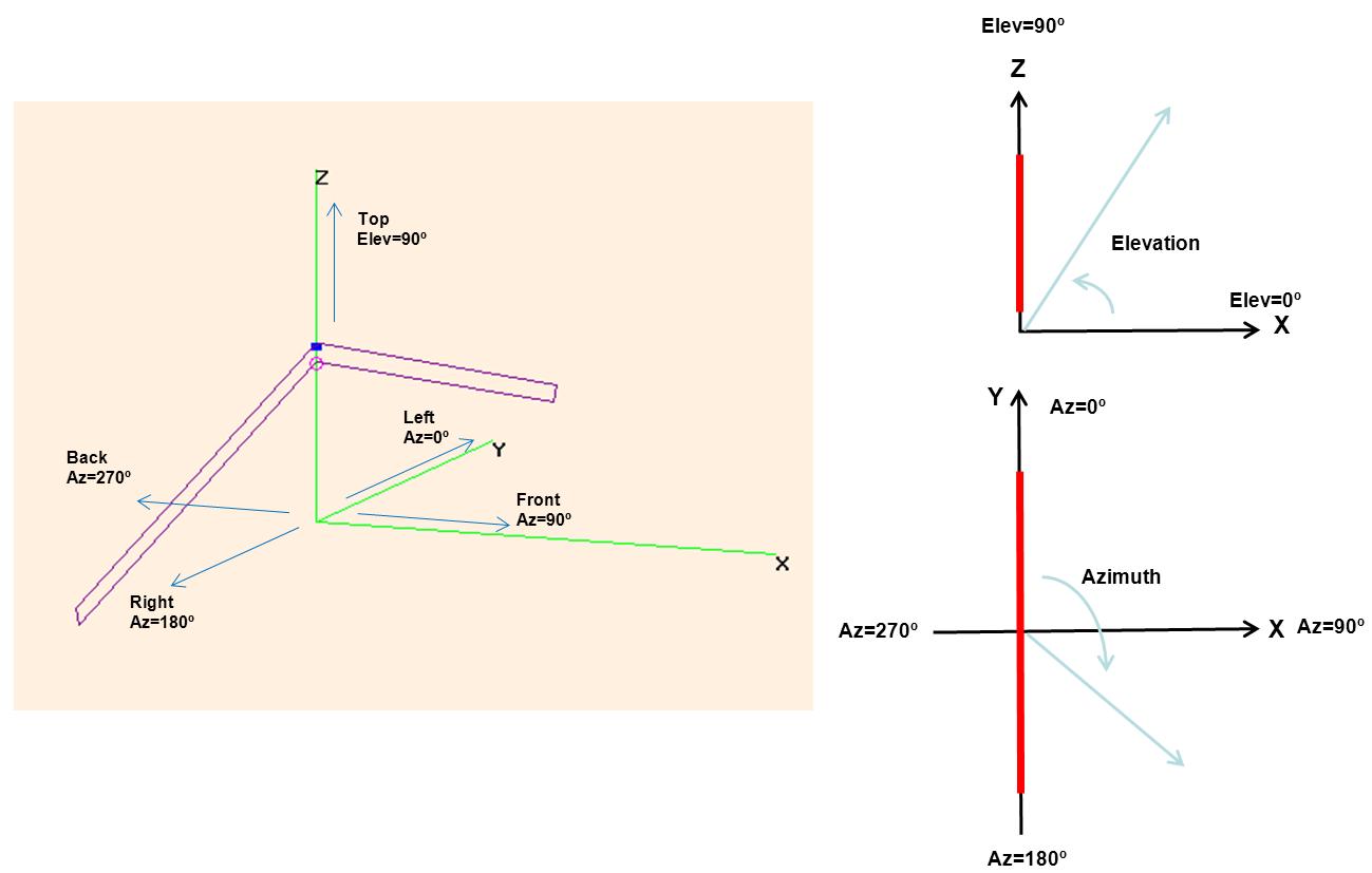
Fig. 2. Conventions used in the simulations.
In this system, the following conventions are used:
-
The ground is defined by the XY plane.
-
The antenna is installed along the Y axis.
-
The height is measured along the Z axis.
-
The takeoff angle is measured from the ground (XY plane) towards the positive Z semi-axis, with possible values between 0º (ground) and 90º (direction perpendicular to the ground).
-
The azimuth angle is measured from the positive Y semi-axis towards the positive X semi-axis, with possible values between 0º and 360º. Thus, the different directions of interest are:
-
Azimuth = 0º: left side of the antenna.
-
Azimuth = 90º: front side of the antenna.
-
Azimuth = 180º: right side of the antenna.
-
Azimuth = 270º: back side of the antenna.
The mast of the antenna is not simulated in any case, so it is necessary to take into account that in a real installation it will affect both the impedance and the radiation patterns of the antenna with respect to the results of the simulations.
2.1. Model 1.
Fig. 3 shows the first model used to simulate the antenna in 4NEC2. Click on the image to see a larger version.
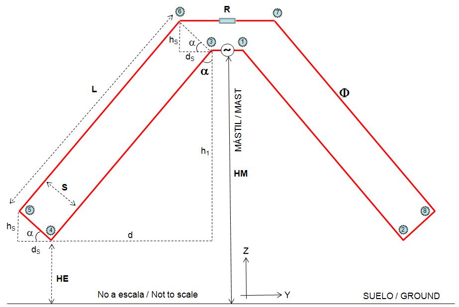
Fig. 3. Model 1.
The wires of the model are numbered as shown in Table 1.
| Wire | End 1 | End 2 |
|---|---|---|
| 1 | P1 | P3 |
| 2 | P3 | P4 |
| 3 | P4 | P5 |
| 4 | P5 | P6 |
| 5 | P6 | P7 |
| 6 | P7 | P8 |
| 7 | P8 | P2 |
| 8 | P2 | P1 |
Table 1. Wires of the model 1.
To determine the coordinates of the eight points defining each section of the model, the following trigonometric relationships are used:
On the other and and as stated before, the height of installation of the tips of the antenna (HE) can be computed using the height of the mast (HM) and the semi-angle formed by the legs of the antenna (α). The same way, the angle α can be computed using HM and HE, using the following formula. Remember that α is half the angle formed by the two legs of the antenna. This way, an angle α = 90º means that the antenna is installed horizontally.
In this model, a horizontal section of 0,5 m in length (wire 1) is used to install the generator, placed at a height HM (height of the mast). This is the point of installation of the balun in the real antenna. This additional section of the model is necessary to avoid having the generator on the tip of one of the wires, a configuration which may cause errors in the results obtained with the NEC-2 algorithm.
The antenna is deployed in inverted-vee configuration, being its tips at a height HE over the ground. On each leg, the sections of the antenna between the two main wires (wires 3 and 7, length S) are arranged perpendicular to them. Finally, the model includes another horizontal section of variable length on the top (wire 5) to place the resistive load. In this model I have considered that the two main wires of each leg have the same length L. Notice that using this model in inverted-vee configuration, the two horizontal wires (1 and 5) are separated a length slightly lower than S.
Using the draw and the trigonometric relations presented before, the coordinates of the 8 points of interest will be:
2.2. Model 2.
Fig. 4 shows the second model used to simulate the antenna in 4NEC2. Click on the image to see a larger version.
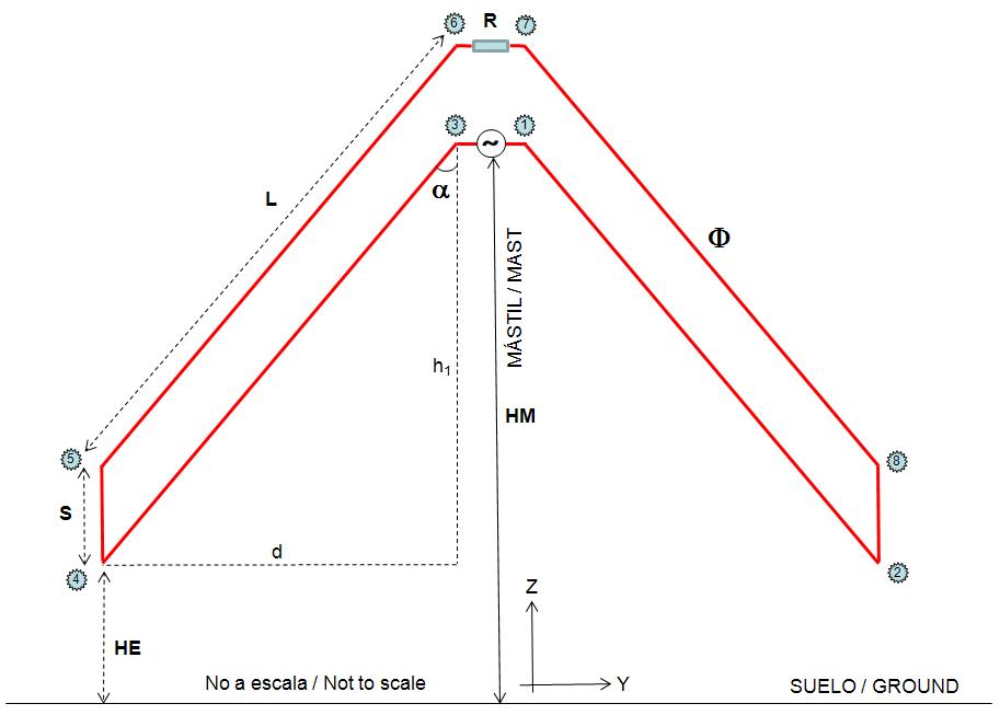
Fig. 4. Model 2.
The wires of the model are numbered as shown in the table 2.
| Wire | End 1 | End 2 |
|---|---|---|
| 1 | P1 | P3 |
| 2 | P3 | P4 |
| 3 | P4 | P5 |
| 4 | P5 | P6 |
| 5 | P6 | P7 |
| 6 | P7 | P8 |
| 7 | P8 | P2 |
| 8 | P2 | P1 |
Table 2. Wires of the model 2.
In this model, a horizontal section of 0,5 m in length (wire 1) is used to install the generator, placed at a height HM (height of the mast). This is the point of installation of the balun in the real antenna. This additional section of the model is necessary to avoid having the generator on the tip of one of the wires, a configuration which may cause errors in the results obtained with the NEC-2 algorithm.
The antenna is deployed in inverted-vee configuration, being its tips at a height HE over the ground. On each leg, the sections of the antenna between the two main wires (wires 3 and 7, length S) are arranged perpendicular to the ground. Finally, the model includes another horizontal section of variable length on the top (wire 5) to place the resistive load. In this model I have considered that the two main wires of each leg (wires 2-4 and 6-8) have the same length L.
In this case and in contrast to the first model, the two horizontal wires (1 and 5) are always separated a length S.
In order to compute the coordinates of the points of interest, we can use the same trigonometric relations shown in the section 2.1.
Using this model it is necessary to take into account that, if using autosegmentation in 4NEC2, there will be parallel wires with different number of segments, a fact which may have some influence on the results of the simulations.
3. Model validation.
In order to validate the models, I have tried the following inverted-vee configurations of the antenna, simulating masts of different heights (9, 12, 15 and 18 m) and leaving the tips of the antenna at 0,5 m over ground:
-
HM=9, HE=0,5, α=72,32º.
-
HM=12, HE=0,5, α=65,75º.
-
HM=15, HE=0,5, α=58,81º.
-
HM=18, HE=0,5, α=51,31º.
For each model described and using those four configurations, I have made the following tests: geometric check, segment check, convergence test and average gain test (AGT), with the results described in this section.
The geometric and segment checks have been done in the limits of the band (2 MHz and 30 MHz).
The convergency and average gain tests have been done in the following discrete frequencies: 2 MHz, 5 MHz, 10 MHz, 15 MHz, 20 MHz, 25 MHz and 30 MHz.
3.1. Model 1.
The results of the validation tests for the first model are described in this section.
3.1.1. Configuration HM=9, HE=0,5, α=72,32º.
I have tried the segment densities shown in the table 3:
| Wire | Description | TEST 1 | TEST 2 | TEST 3 |
|---|---|---|---|---|
| 1 | Wire with generator | 3 | 3 | 3 |
| 2 | Left leg | 56 | 112 | 185 |
| 3 | Separator left leg | 6 | 6 | 6 |
| 4 | Left leg | 56 | 112 | 185 |
| 5 | Wire with load | 3 | 5 | 7 |
| 6 | Right leg | 56 | 112 | 185 |
| 7 | Separator right leg | 6 | 6 | 6 |
| 8 | Right leg | 56 | 112 | 185 |
Table 3. Segment densities tested with the model 1. Antenna height 9 m and 12 m.
Please note that the load R is always placed in the central segment of the wire (different on each case).
Using the configuration TEST 1, I have achieved AGT values between 1,01 and 1,02 for all the frequencies simulated. Using the configurations TEST 2 and TEST 3, the AGT results 1,00 (very precise model). After performing the convergence test, the configuration TEST 3 is finally chosen.
3.1.2. Configuration HM=12, HE=0,5, α=65,75º.
I have tried the same segment densities described in the table 3.
Using the configuration TEST 1, The simulation yielded an AGT value of 1,01 for all the frequencies simulated. Using the configurations TEST 2 and TEST 3, the AGT results 1,00 (very precise model). After performing the convergence test, the configuration TEST 3 is finally chosen.
3.1.3. Configuration HM=15, HE=0,5, α=58,81º.
I have tried the segment densities shown in the table 4:
| Wire | Description | TEST 1 | TEST 2 | TEST 3 |
|---|---|---|---|---|
| 1 | Wire with generator | 3 | 3 | 3 |
| 2 | Left leg | 56 | 112 | 185 |
| 3 | Separator left leg | 6 | 6 | 6 |
| 4 | Left leg | 56 | 112 | 185 |
| 5 | Wire with load | 3 | 7 | 7 |
| 6 | Right leg | 56 | 112 | 185 |
| 7 | Separator right leg | 6 | 6 | 6 |
| 8 | Right leg | 56 | 112 | 185 |
Table 4. Segment densities tested with the model 1. Antenna height 15 m.
Using the configuration TEST 1, The simulation yielded an AGT value of 1,01 for all the frequencies simulated. Using the configurations TEST 2 and TEST 3, the AGT results 1,00 (very precise model). After performing the convergence test, the configuration TEST 3 is finally chosen.
3.1.4. Configuration HM=18, HE=0,5, α=51,31º.
I have tried the segment densities shown in the table 5:
| Wire | Description | TEST 1 | TEST 2 | TEST 3 |
|---|---|---|---|---|
| 1 | Wire with generator | 3 | 3 | 3 |
| 2 | Left leg | 56 | 112 | 185 |
| 3 | Separator left leg | 6 | 6 | 6 |
| 4 | Left leg | 56 | 112 | 185 |
| 5 | Wire with load | 3 | 7 | 11 |
| 6 | Right leg | 56 | 112 | 185 |
| 7 | Separator right leg | 6 | 6 | 6 |
| 8 | Right leg | 56 | 112 | 185 |
Table 5. Segment densities tested with the model 1. Antenna height 18 m.
Using the configuration TEST 1, The simulation yielded an AGT value of 1,01 for all the frequencies simulated. Using the configurations TEST 2 and TEST 3, the AGT results 1,00 (very precise model). After performing the convergence test, the configuration TEST 3 is finally chosen.
3.2. Model 2.
The results of the validation tests for the second model are described in this section. Due to the fact that in this model all the wires have the same lengths with independence of the configuration used to install the antenna, I have tested the segment densities shown in the table 6, which are valid for all the cases.
| Wire | Description | TEST 1 | TEST 2 | TEST 3 |
|---|---|---|---|---|
| 1 | Wire with generator | 3 | 3 | 3 |
| 2 | Left leg | 56 | 112 | 186 |
| 3 | Separator left leg | 6 | 6 | 6 |
| 4 | Left leg | 56 | 112 | 186 |
| 5 | Wire with load | 3 | 3 | 3 |
| 6 | Right leg | 56 | 112 | 186 |
| 7 | Separator right leg | 6 | 6 | 6 |
| 8 | Right leg | 56 | 112 | 186 |
Table 6. Segment densities tested with the model 2.
3.2.1. Configuration HM=9, HE=0,5, α=72,32º.
Using the configuration TEST 1, I have achieved AGT values between 1,01 and 1,02 for all the frequencies simulated. Using the configurations TEST 2 and TEST 3, the AGT results 1,00 (very precise model).
The segment validation tests performed with the configurations TEST 1 and TEST 2 show a warning indicating misalignment of some parallel segments at 5 MHz.
After performing the convergence test, the configuration TEST 2 is finally chosen.
3.2.2. Configuration HM=12, HE=0,5, α=65,75º.
Using the configuration TEST 1, I have achieved AGT values between 1,01 and 1,02 for all the frequencies simulated. Using the configurations TEST 2 and TEST 3, the AGT results 1,00 (very precise model).
The segment validation tests performed with the configurations TEST 1 and TEST 2 show a warning indicating misalignment of some parallel segments at 5 MHz.
After performing the convergence test, the configuration TEST 2 is finally chosen.
3.2.3. Configuration HM=15, HE=0,5, α=58,81º.
Using the configuration TEST 1, I have achieved an AGT value of 1,01 for all the frequencies simulated. Using the configurations TEST 2 and TEST 3, the AGT results 1,00 (very precise model).
The segment validation tests performed with the configuration TEST 3 show a warning indicating misalignment of some parallel segments at 5 MHz.
After performing the convergence test, the configuration TEST 2 is finally chosen.
3.2.4. Configuration HM=18, HE=0,5, α=51,31º.
Using the configuration TEST 1, I have achieved an AGT value of 1,01 for all the frequencies simulated. Using the configurations TEST 2 and TEST 3, the AGT results 1,00 (very precise model).
The segment validation tests performed with the configurations TEST 1 and TEST 2 show a warning indicating misalignment of some parallel segments at 5 MHz.
After performing the convergence test, the configuration TEST 2 is finally chosen.
4. 4NEC2 simulation files.
In this section the 4NEC2 simulation files for both models of the Invelco AT-110 antenna are shown. The values of the parametres L, S, R and phi can be consulted in the antenna's user manual.
CM Invelco AT-110 antenna (folded dipole) |
CM Invelco AT-110 antenna (folded dipole) |
5. Simulation of the AT-110A antenna (model 1).
5. Simulation of the AT-110A antenna (model 1).
In this section I will show the results of the simulations performed with the Invelco AT-110A antenna 4NEC2 model 1, presented in the section 2. The values of L, S, R and φ can be consulted in the antenna's user manual.
In all the simulations, a ground of average type is considered, with a conductivity of 0.005 S/m and a dielectric constant of 13.
I have used discrete frequencies in all the working range of the antenna (2-30 MHz), at 1 MHz intervals or even at 200 kHz intervals when necessary.
On the other hand, the SWR calculations will be referred to a characteristic impedance of 450 ohms (9:1 balun in order to work with 50 ohms radios).
I have simulated configurations with masts of lengths HM equal to 9 m, 12 m, 15 m and 18 m, being for all of them the height of installation of the tips HE equal to 0,5 m. In those four cases, the angle between the two legs of the antena will be of 144º, 131º, 117º and 102º, respectively.
Finally, in all the simulations a resolution of 1 degree will be used.
5.1. Computation of the standing wave ratio (SWR).
Fig. 5 shows the SWR vs frequency plots resulting from the simulations of the model 1. Click on the image to see a larger version.
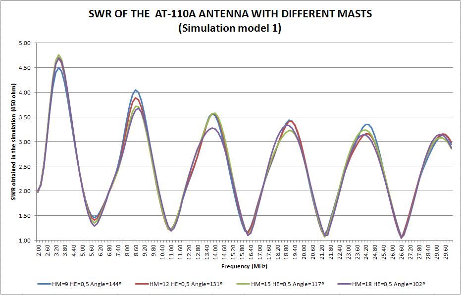
Fig. 5. SWR of the AT-110A antenna with different masts. Simulation model 1.
The results will be analysed in the section 7.
5.2. Simulation of radiation patterns.
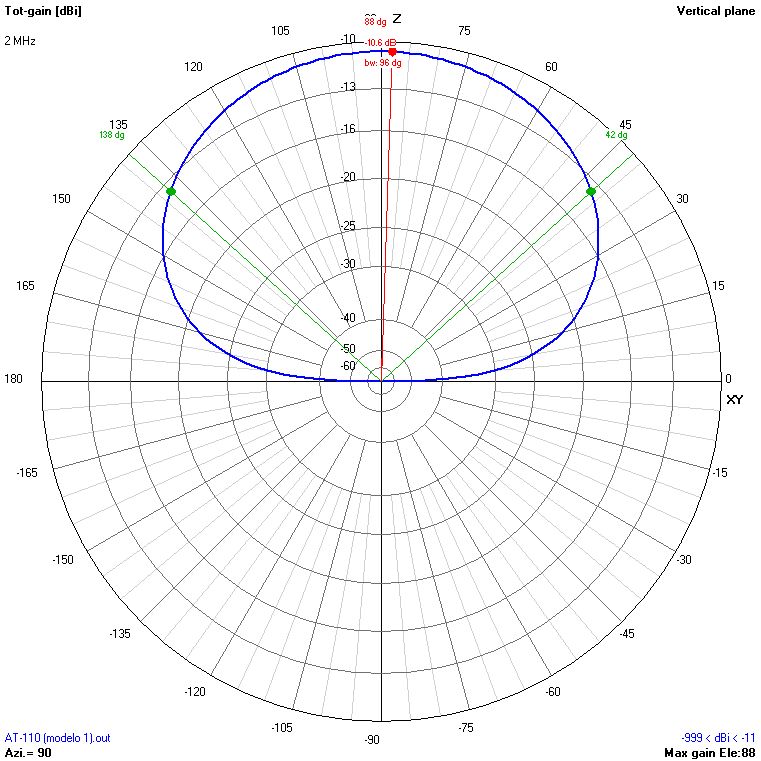
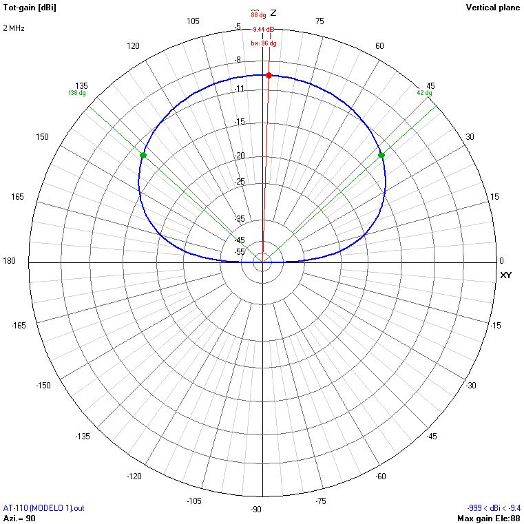
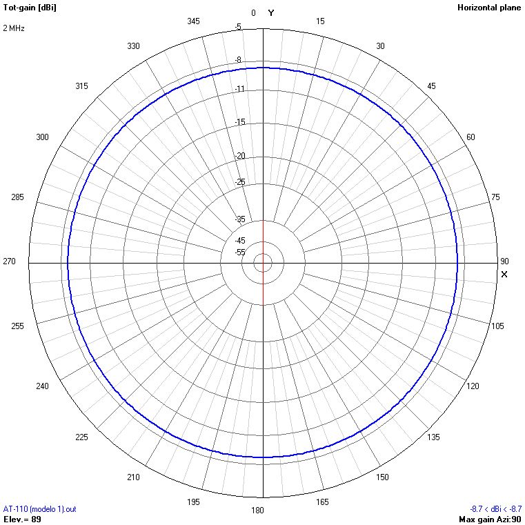
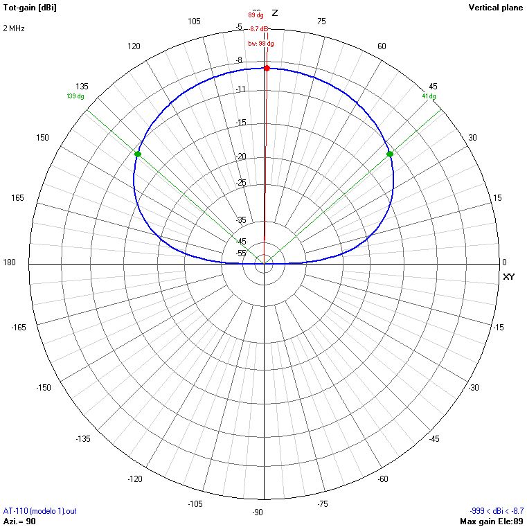
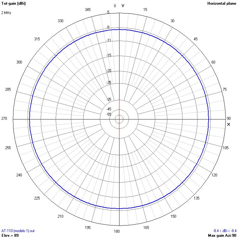
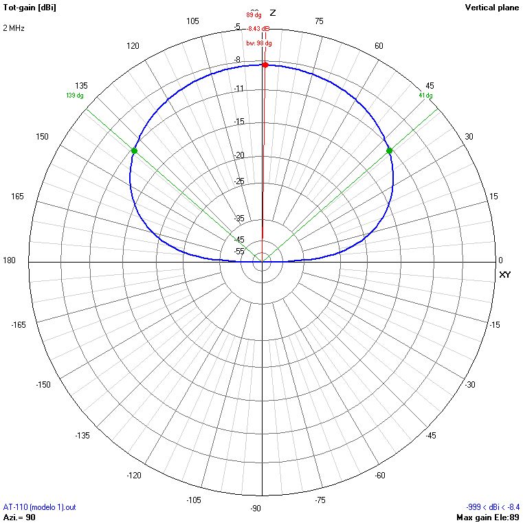
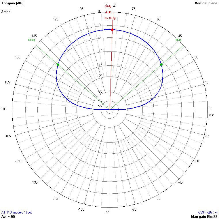
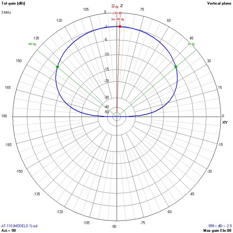
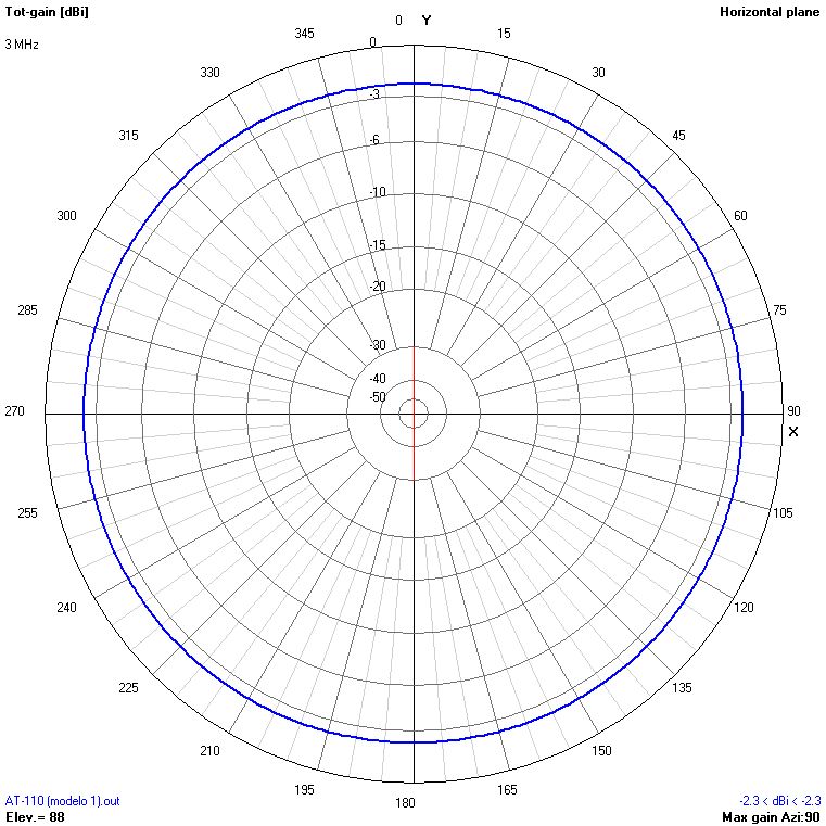
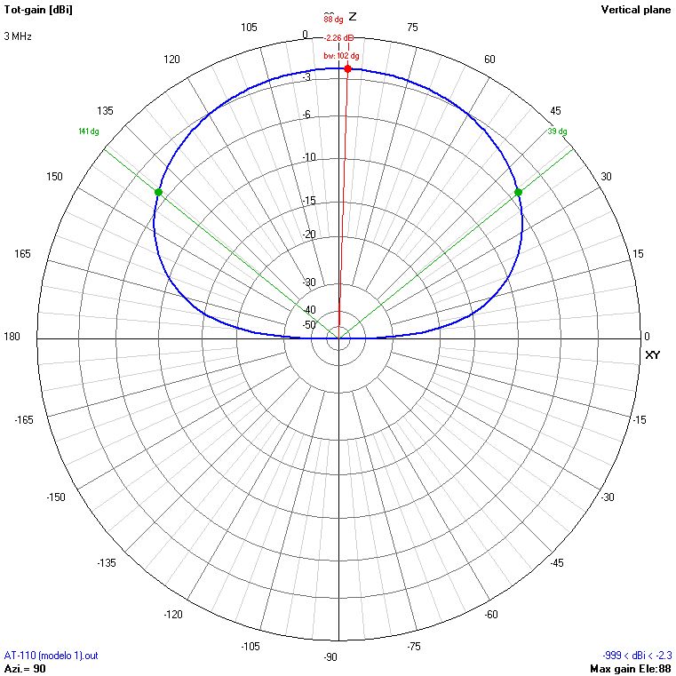
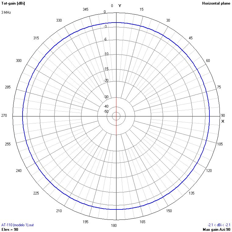
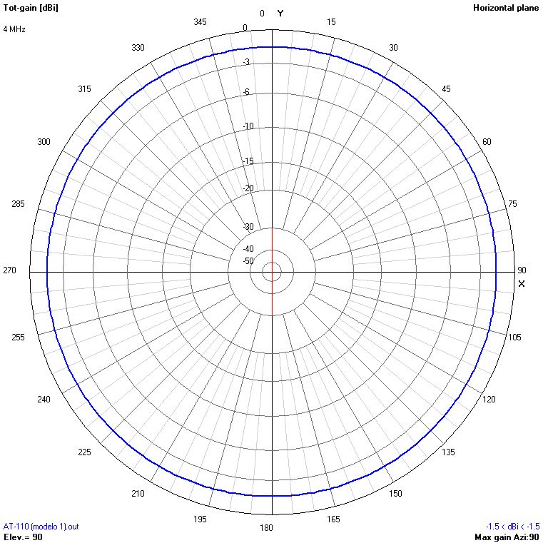
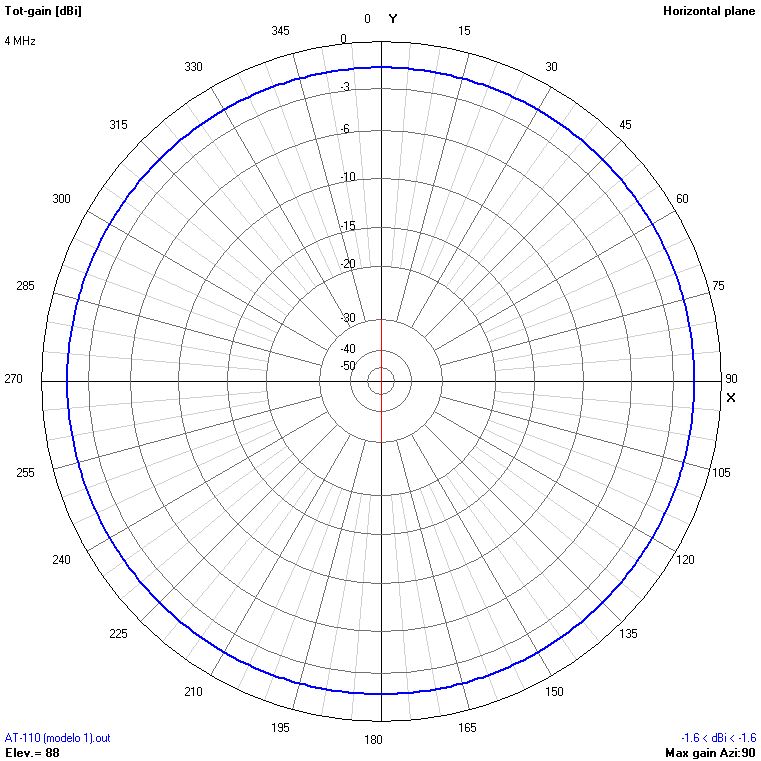
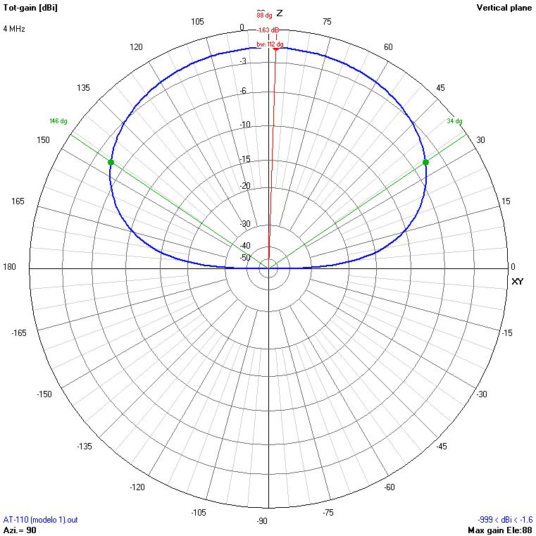
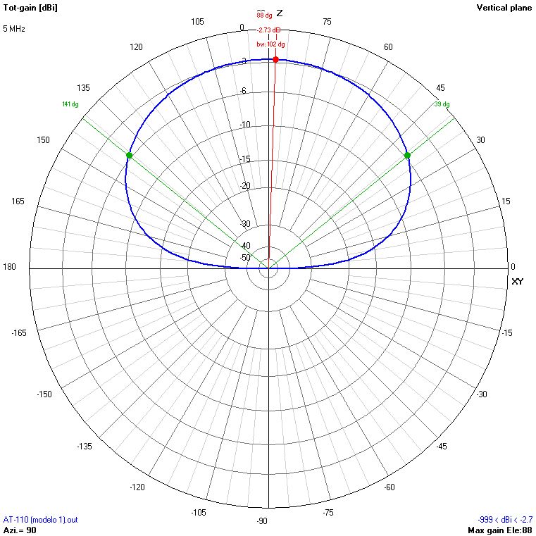
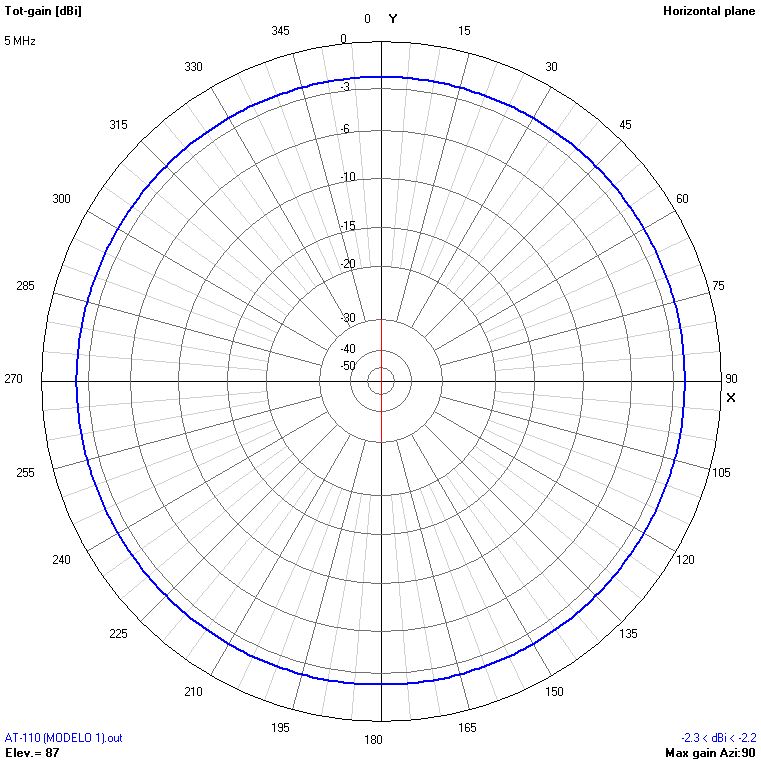
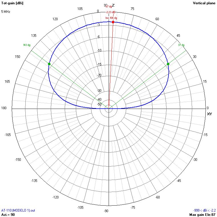
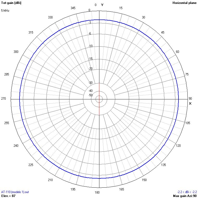
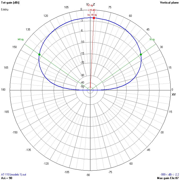
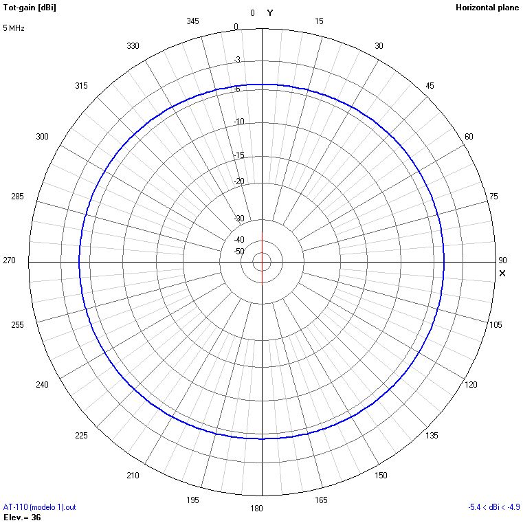
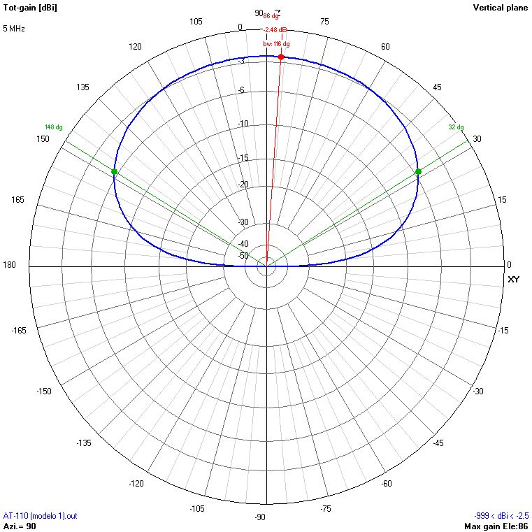
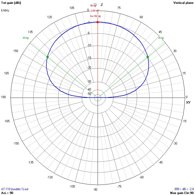
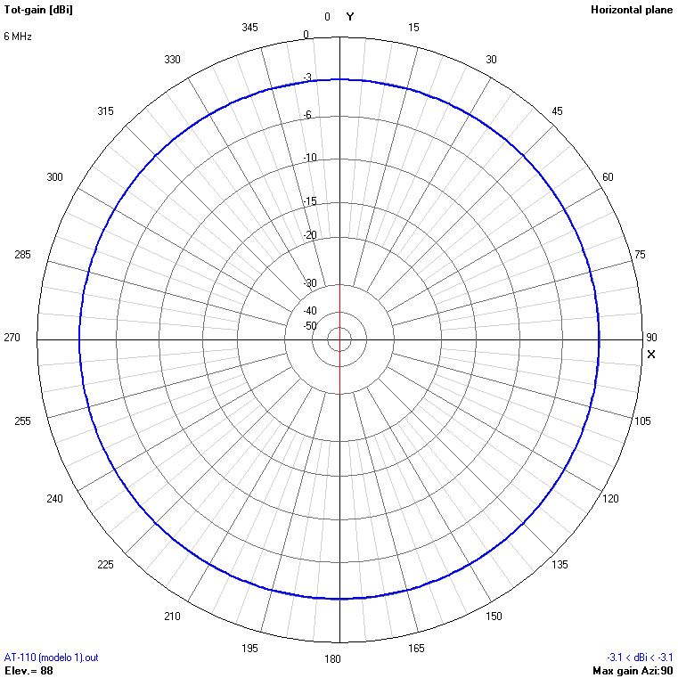
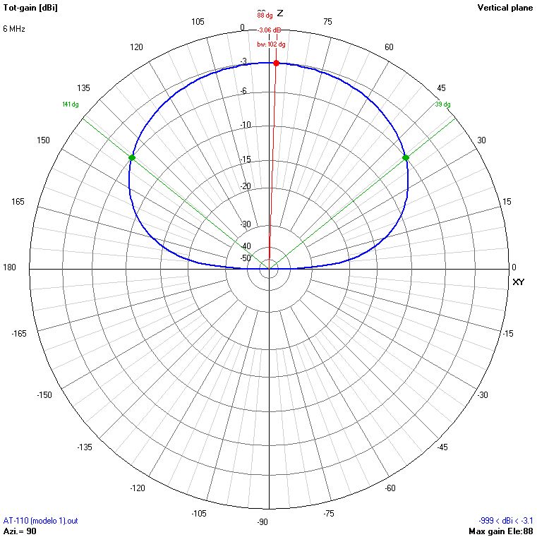
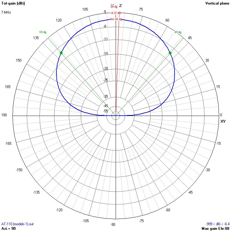
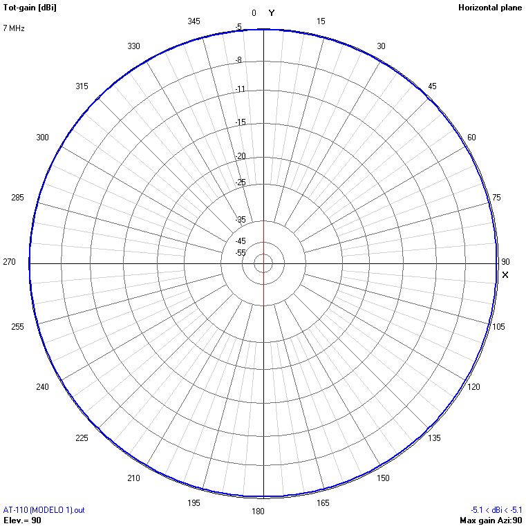
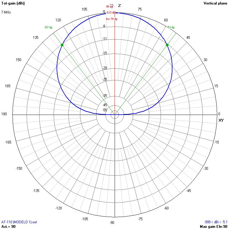
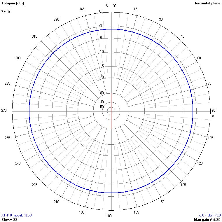
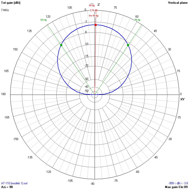
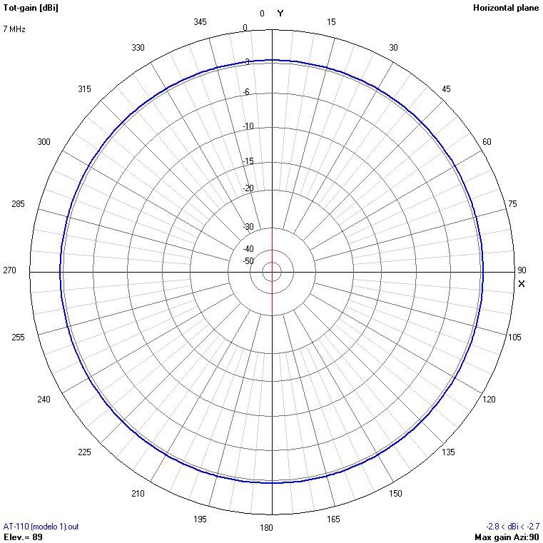
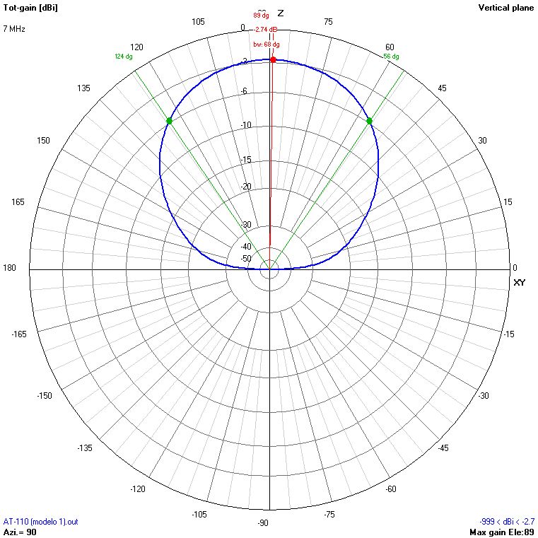
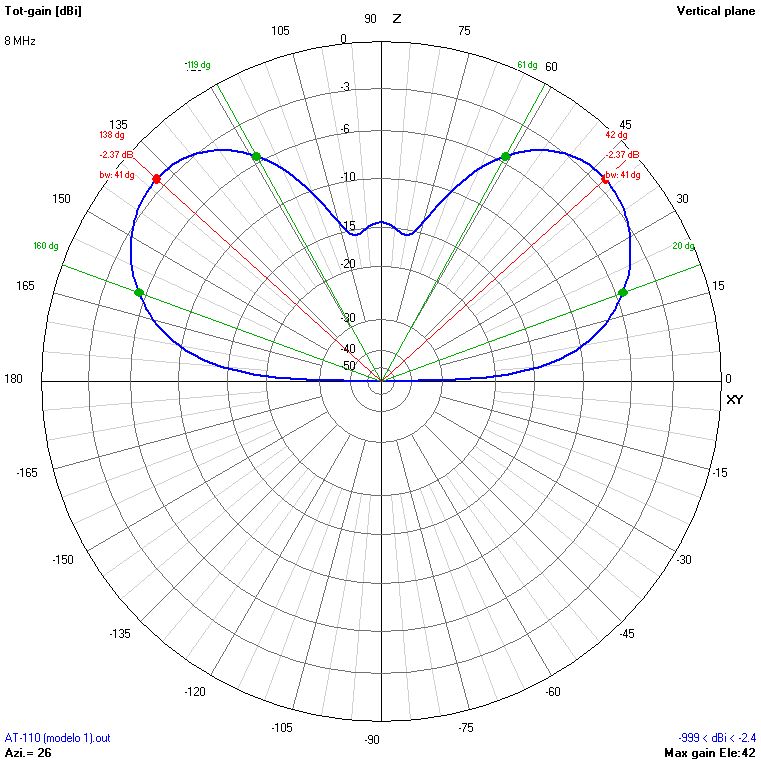
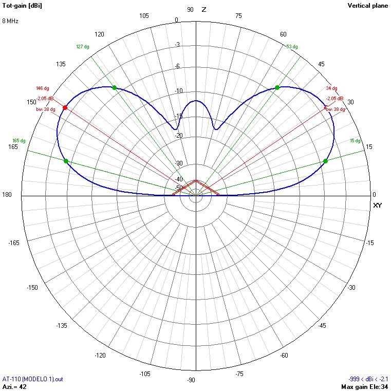
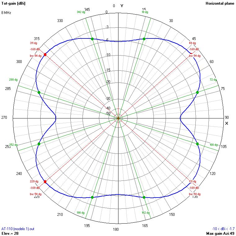
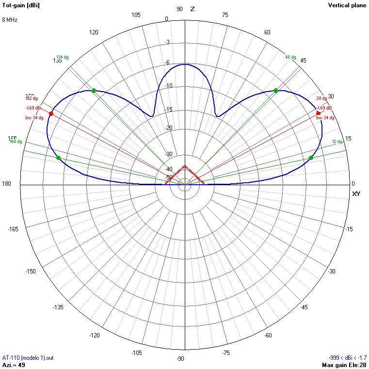
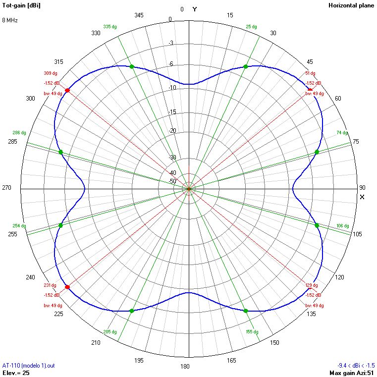
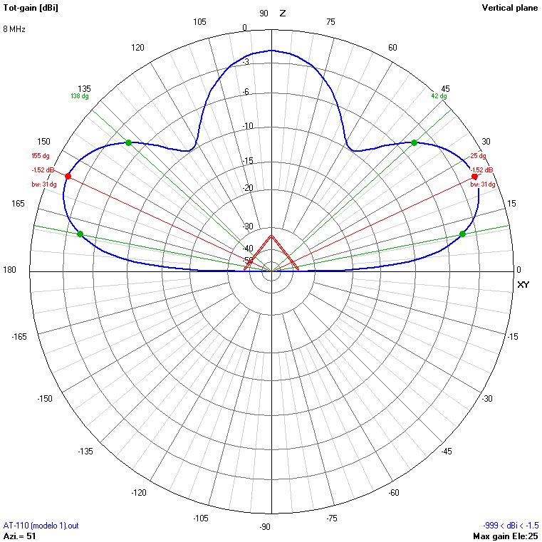
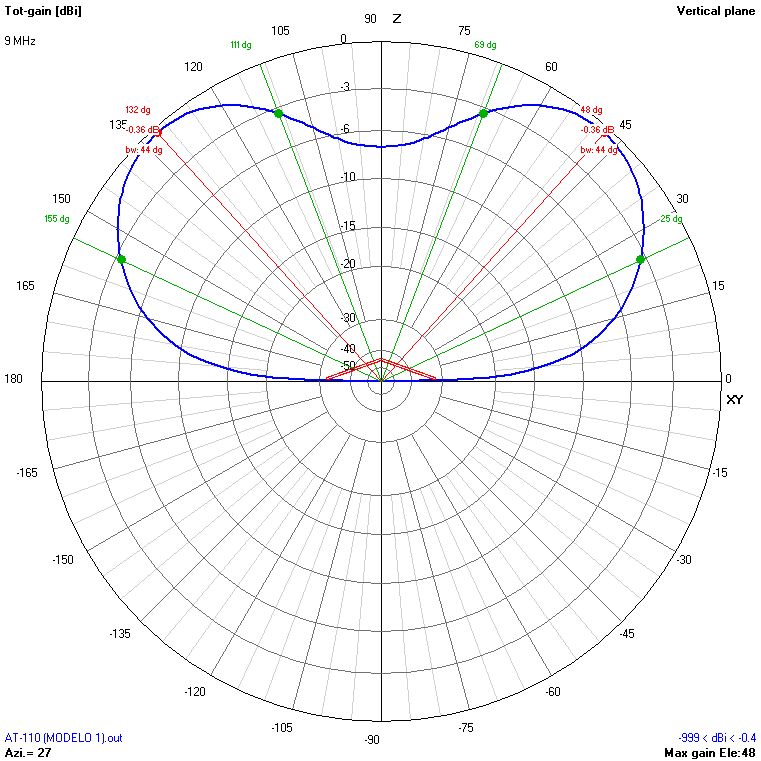
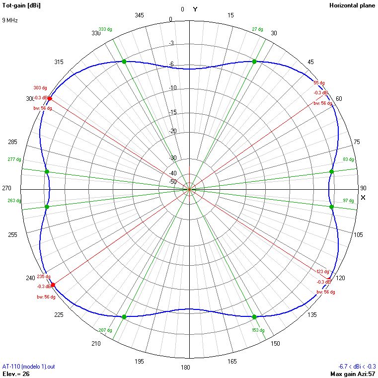
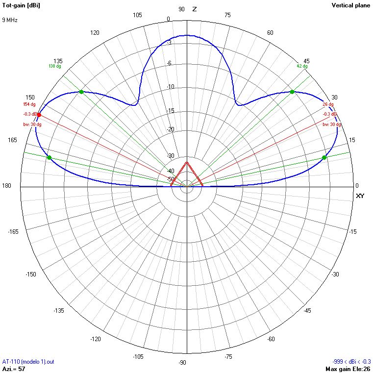
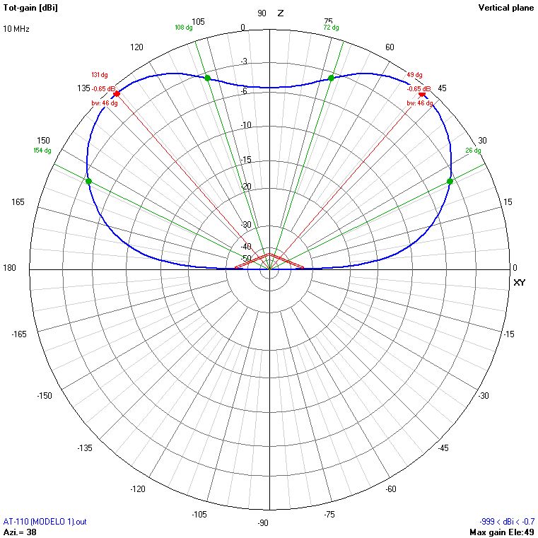
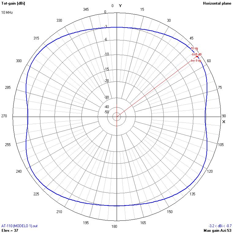
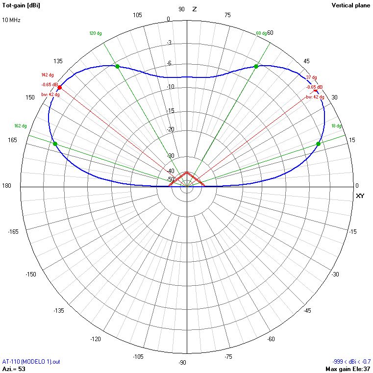
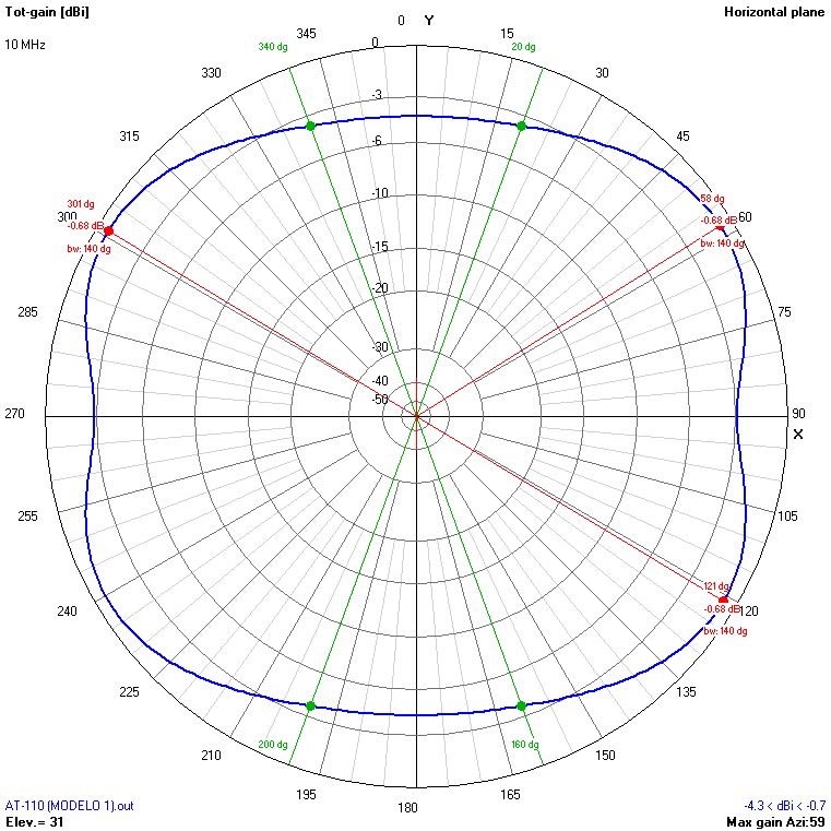
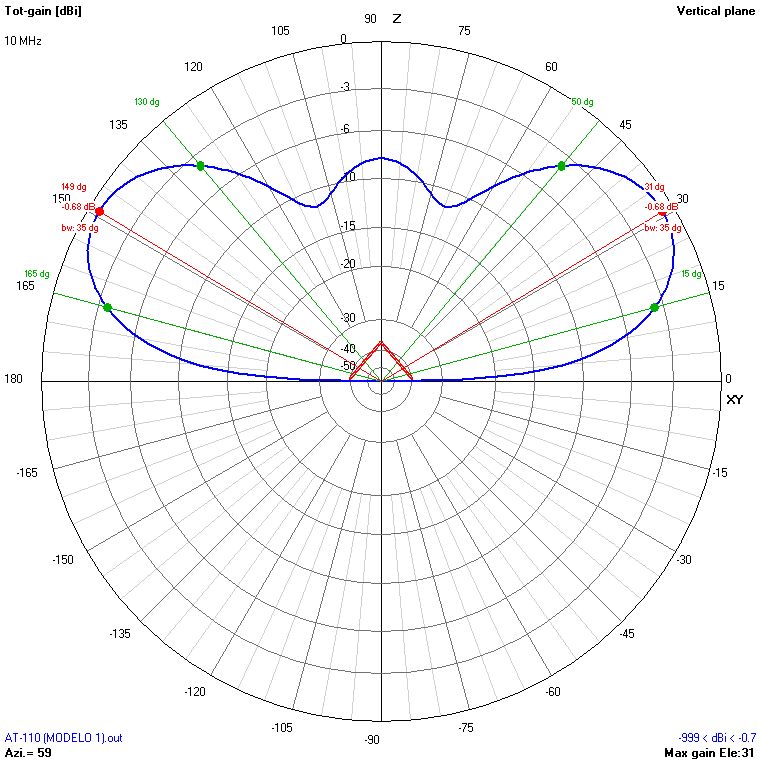
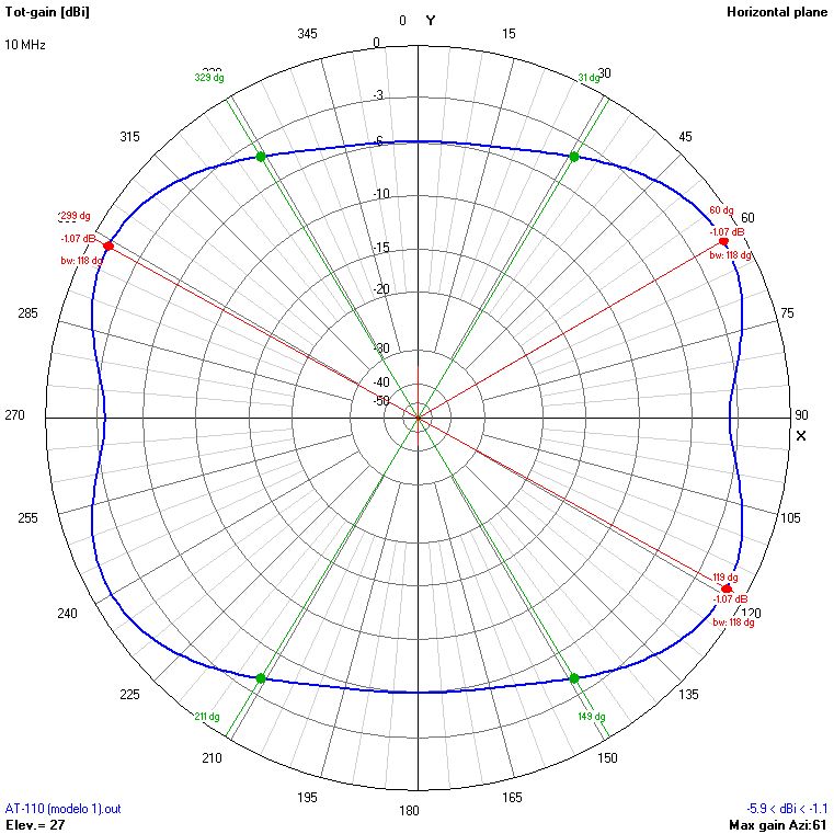
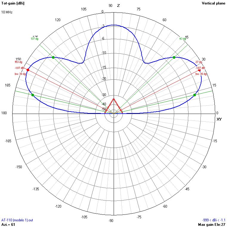
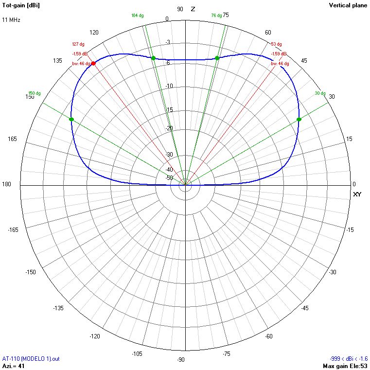
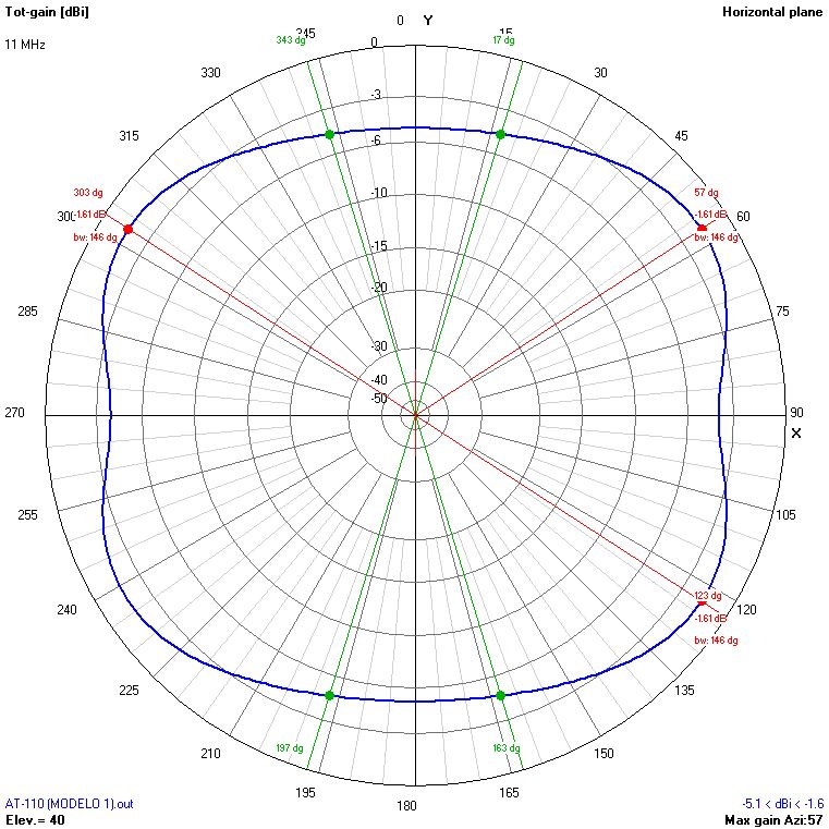
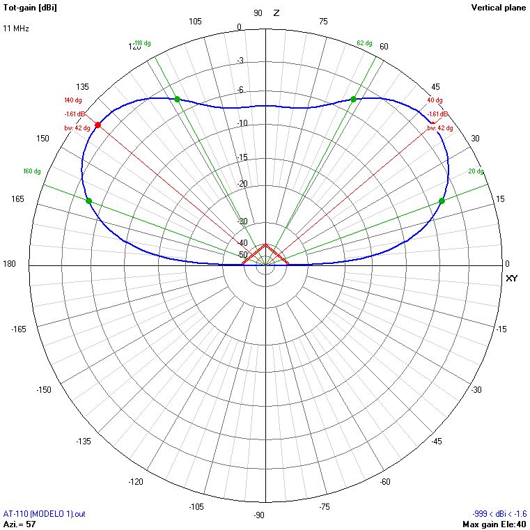
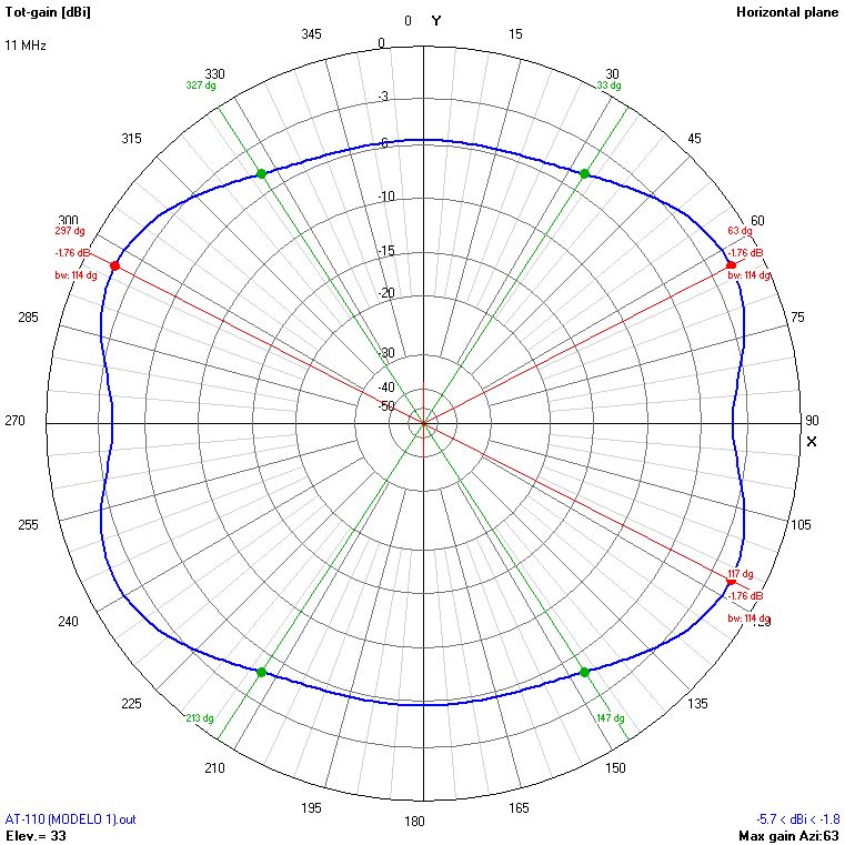
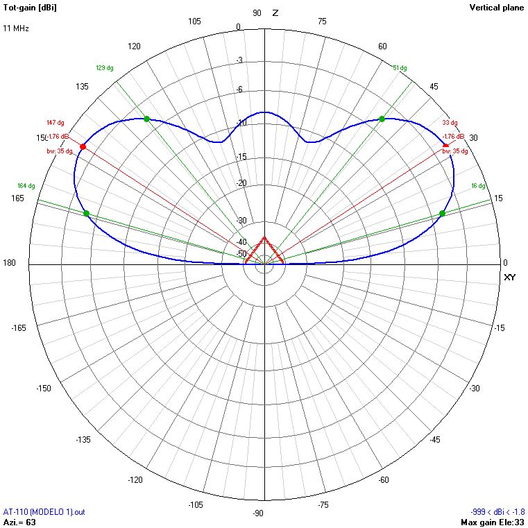
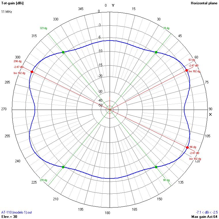
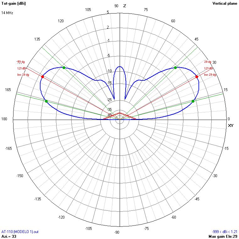
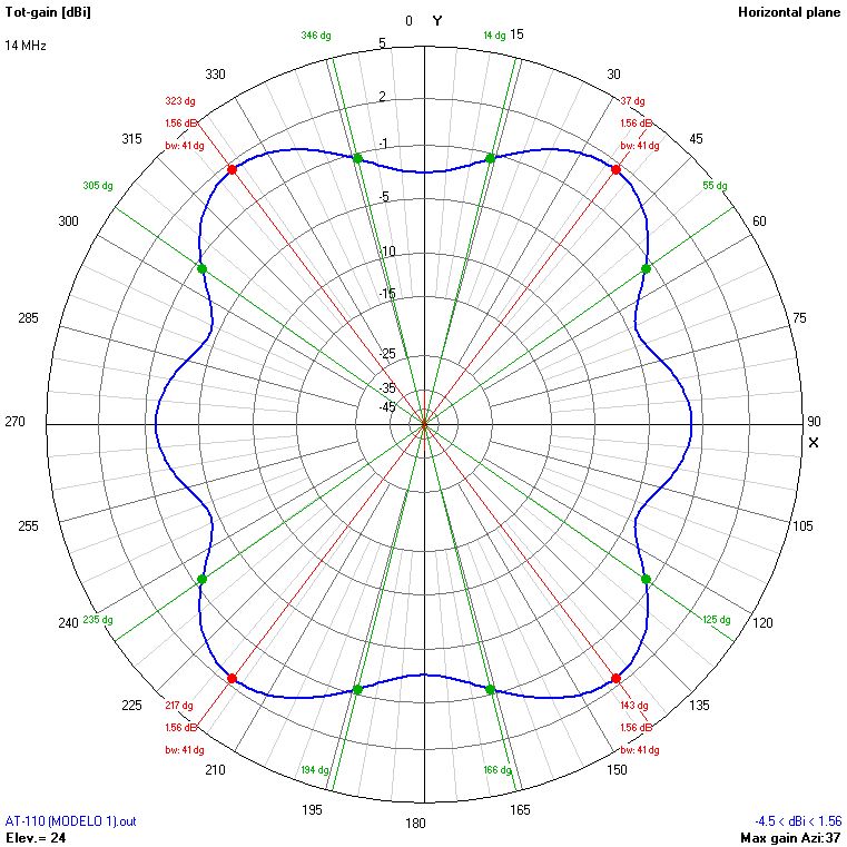
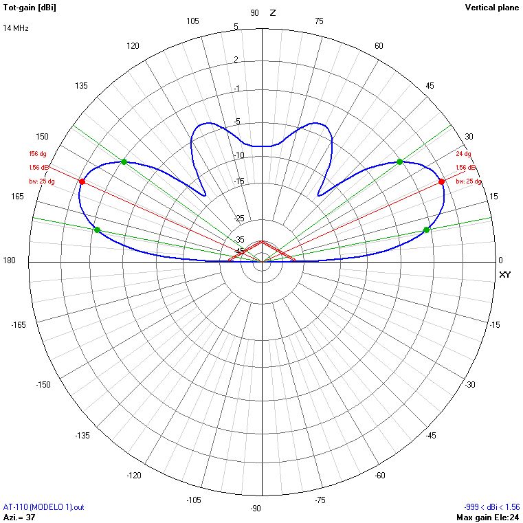
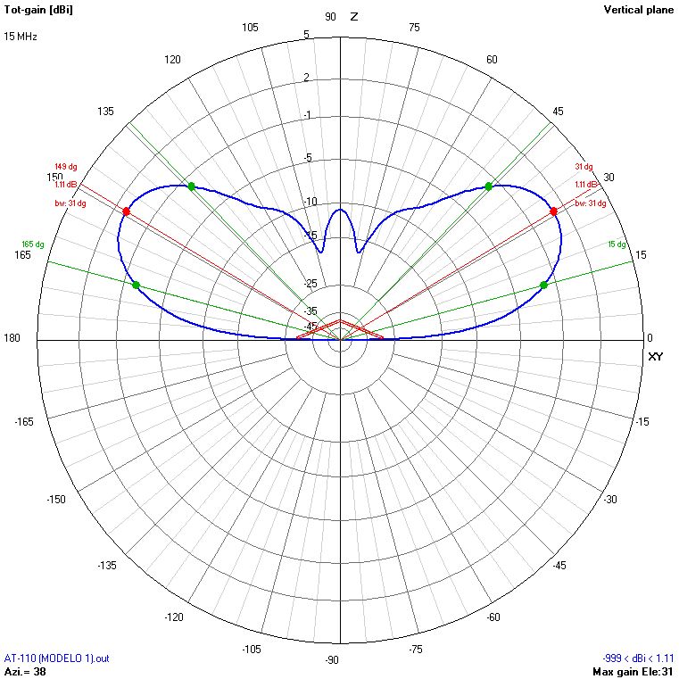
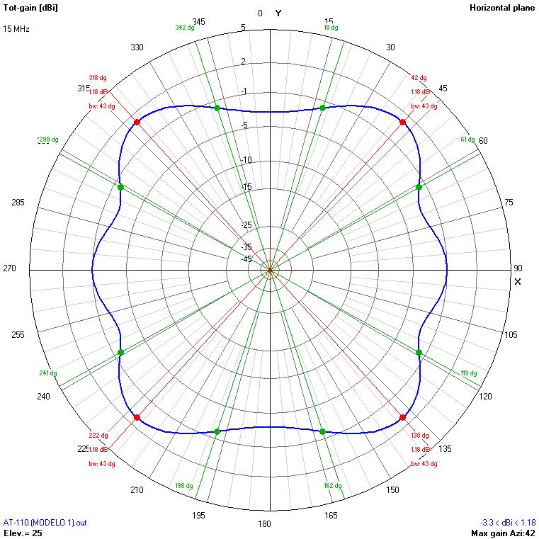
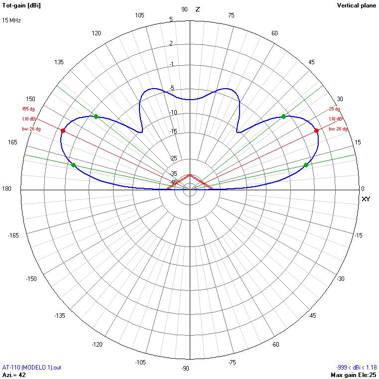
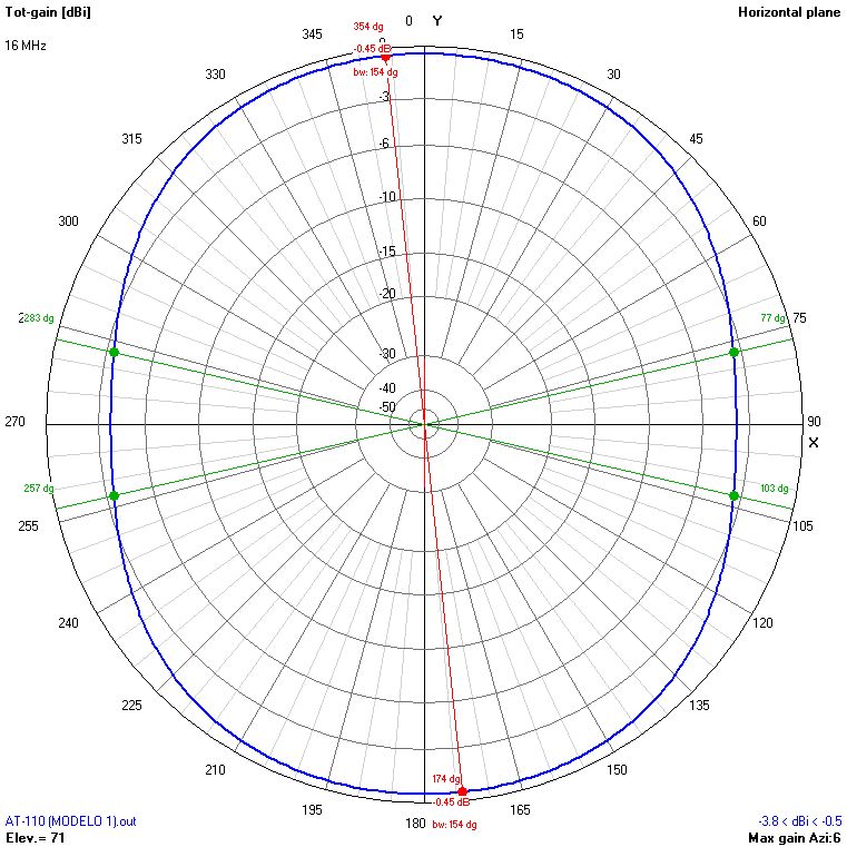
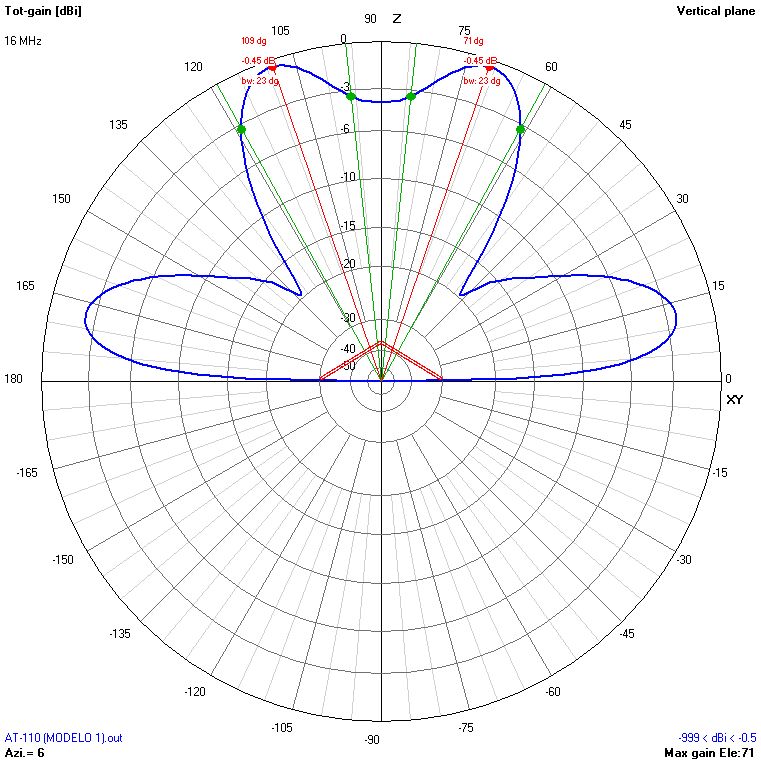
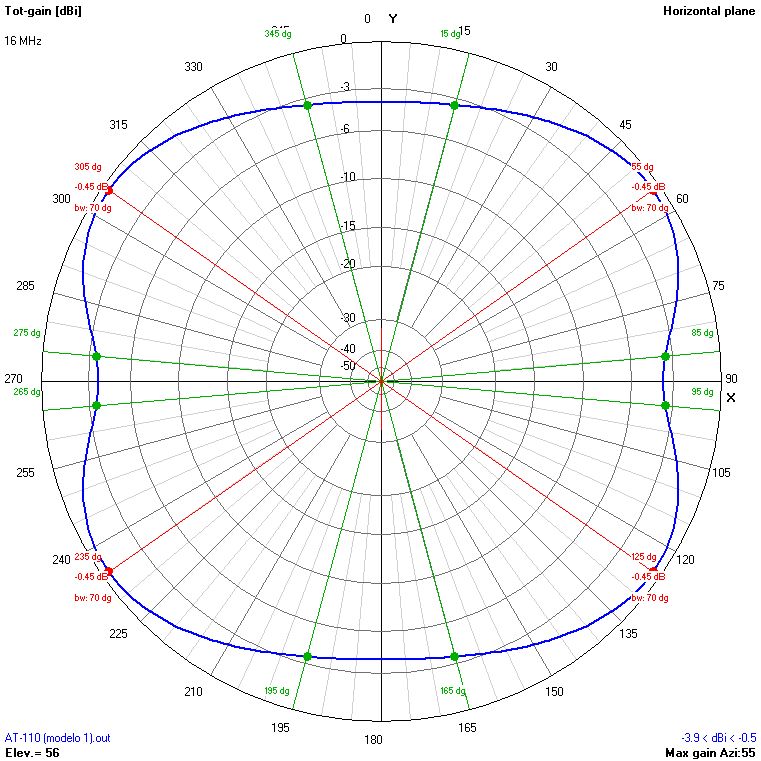
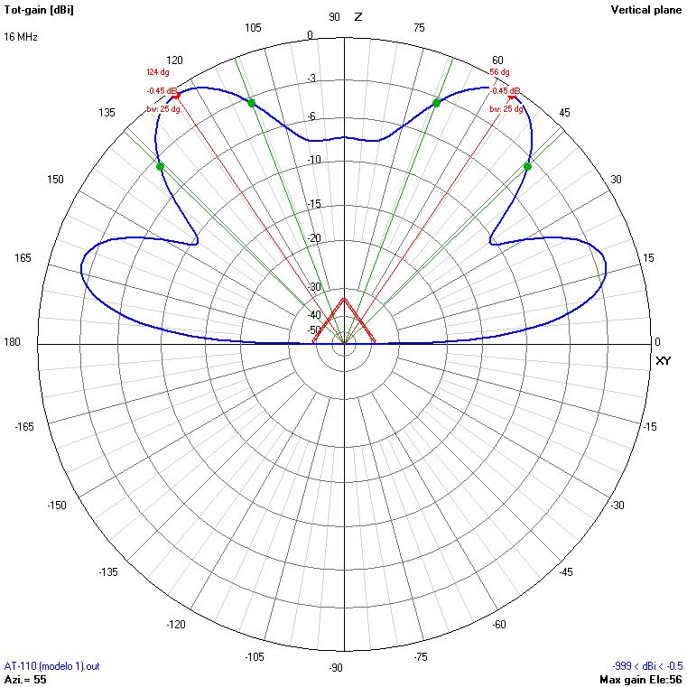
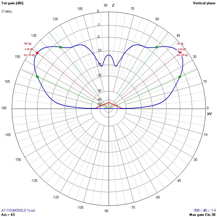
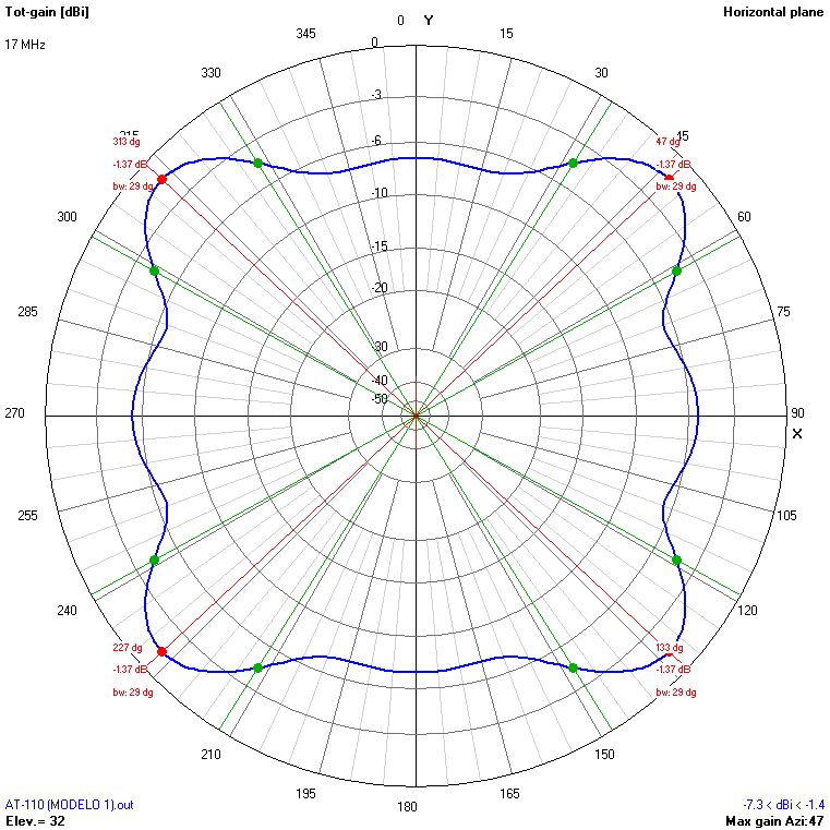
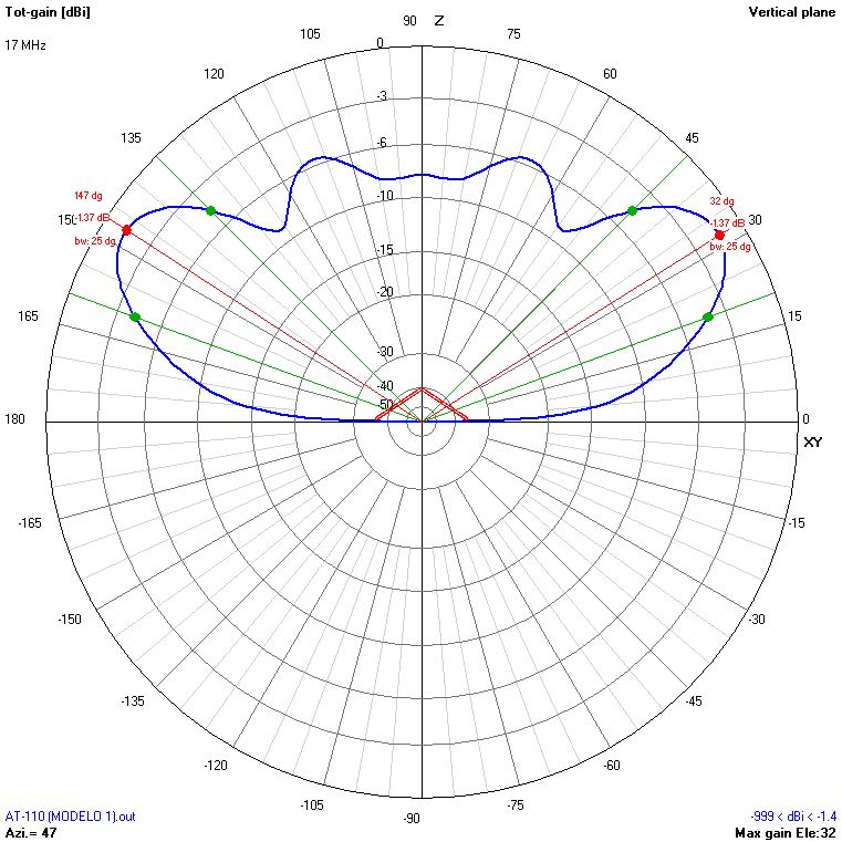
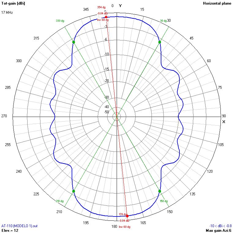
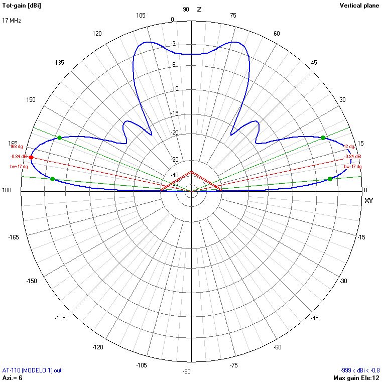
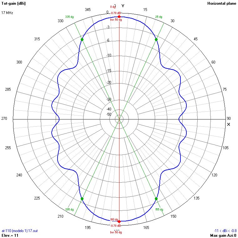
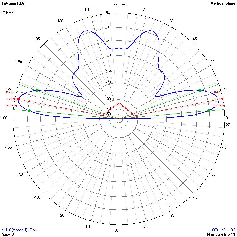
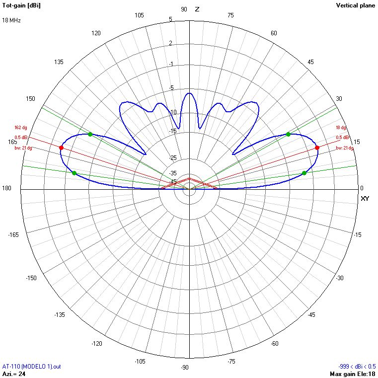
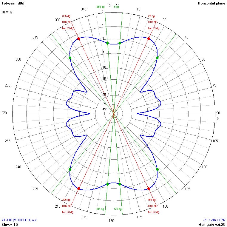
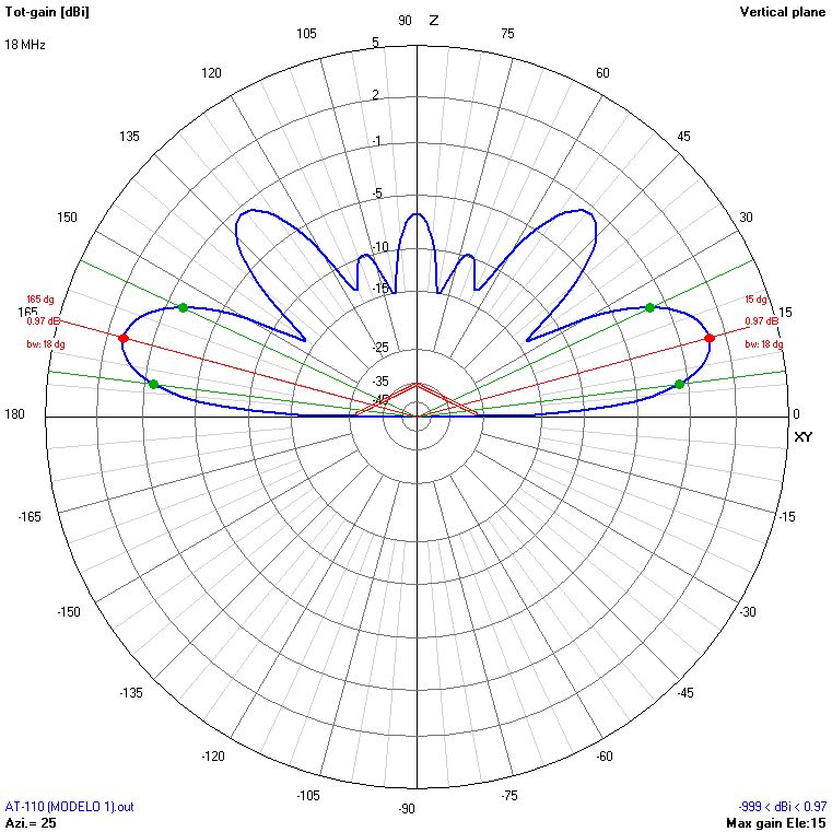
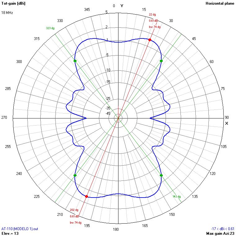
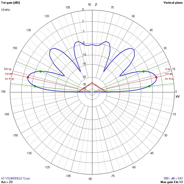
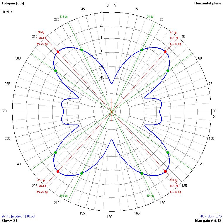
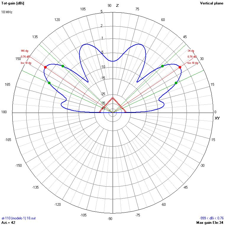
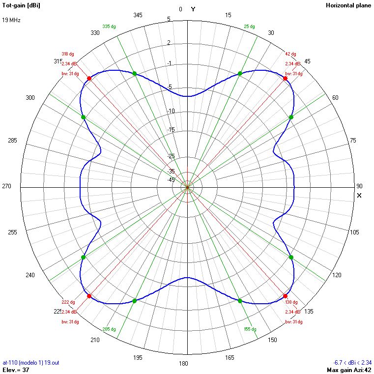
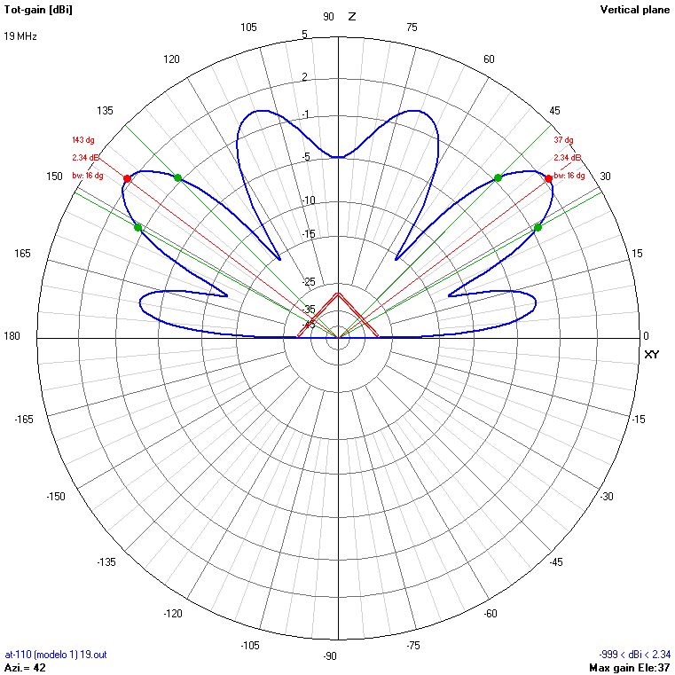
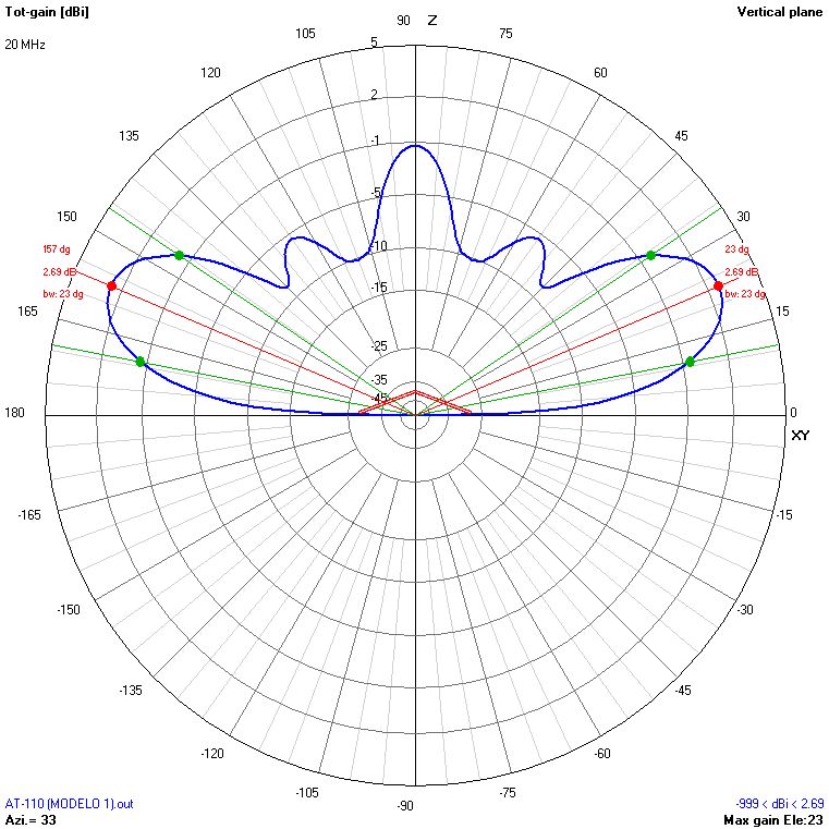
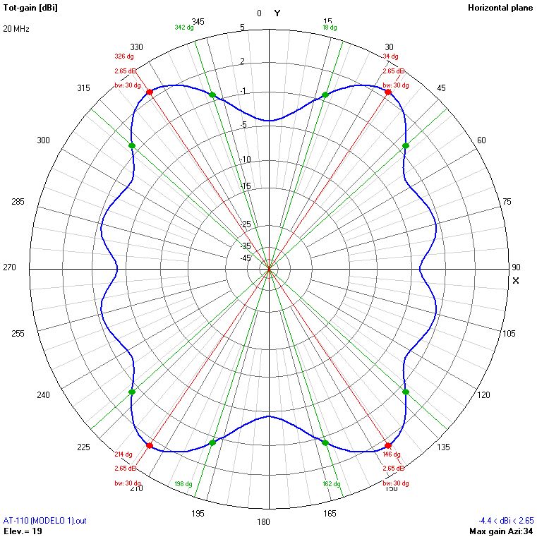
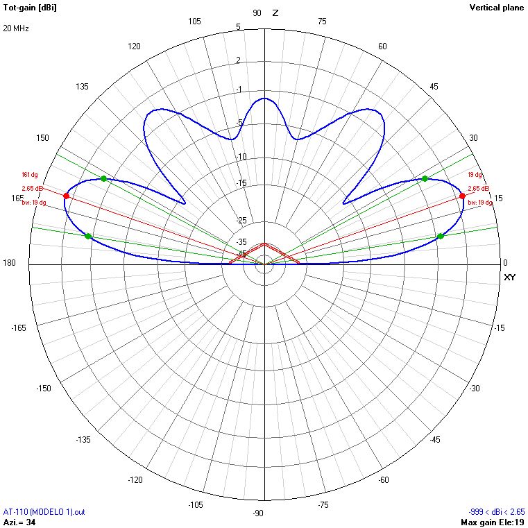
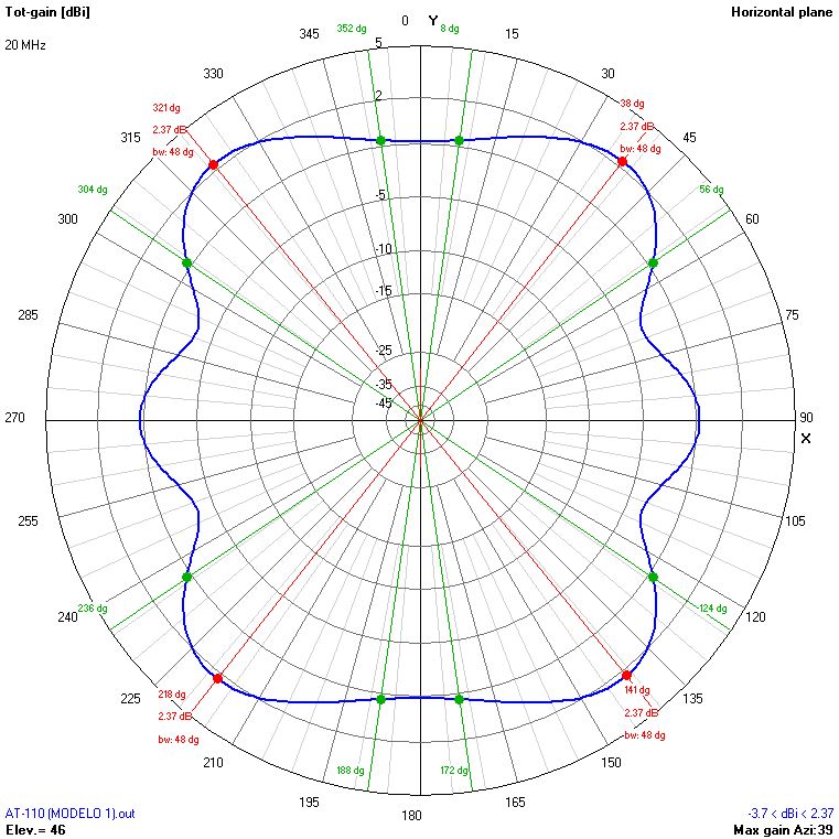
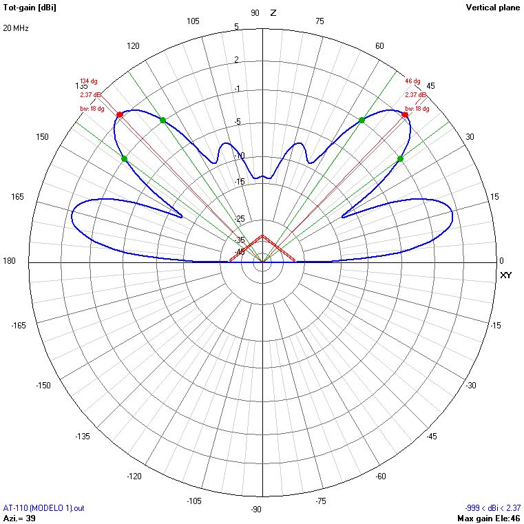
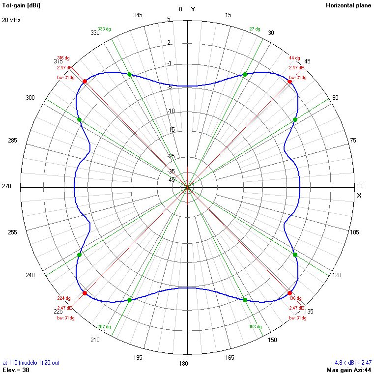
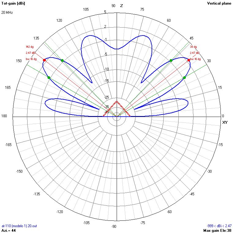
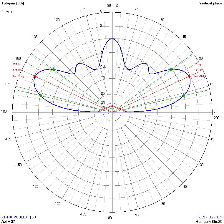
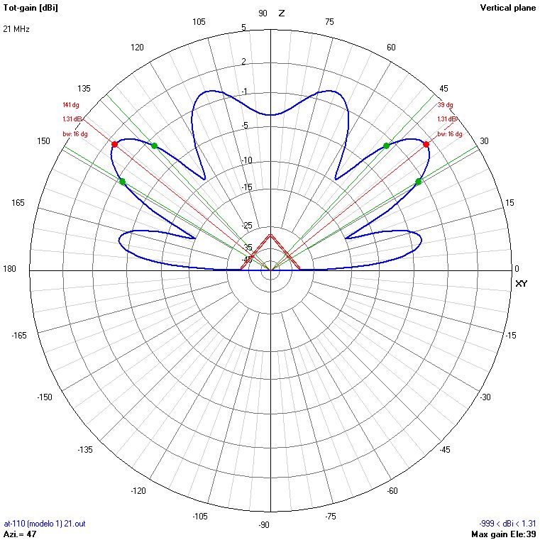
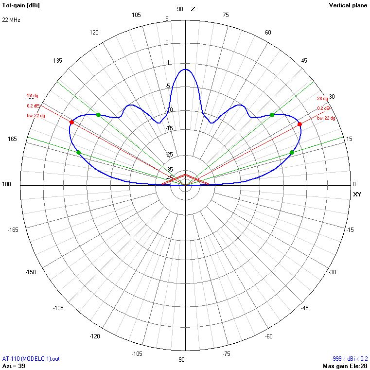
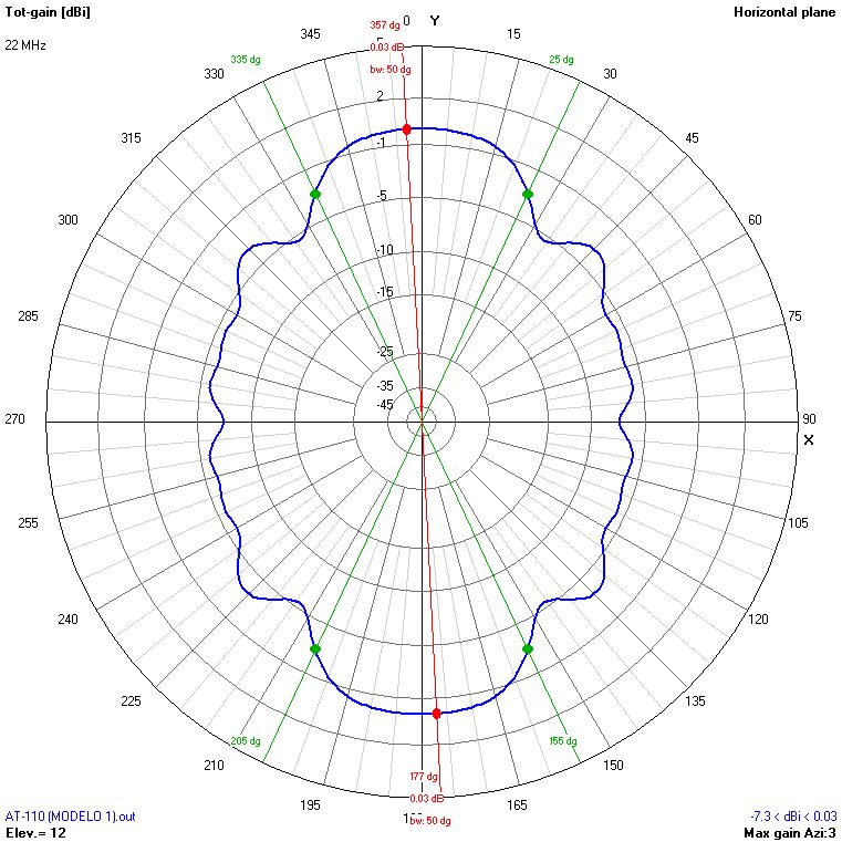
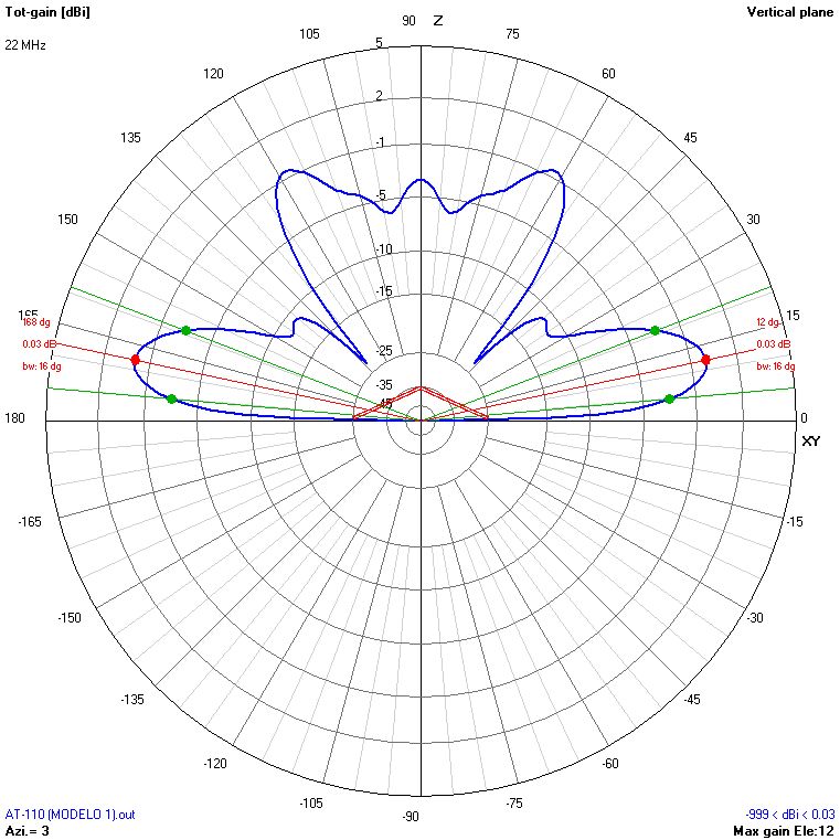
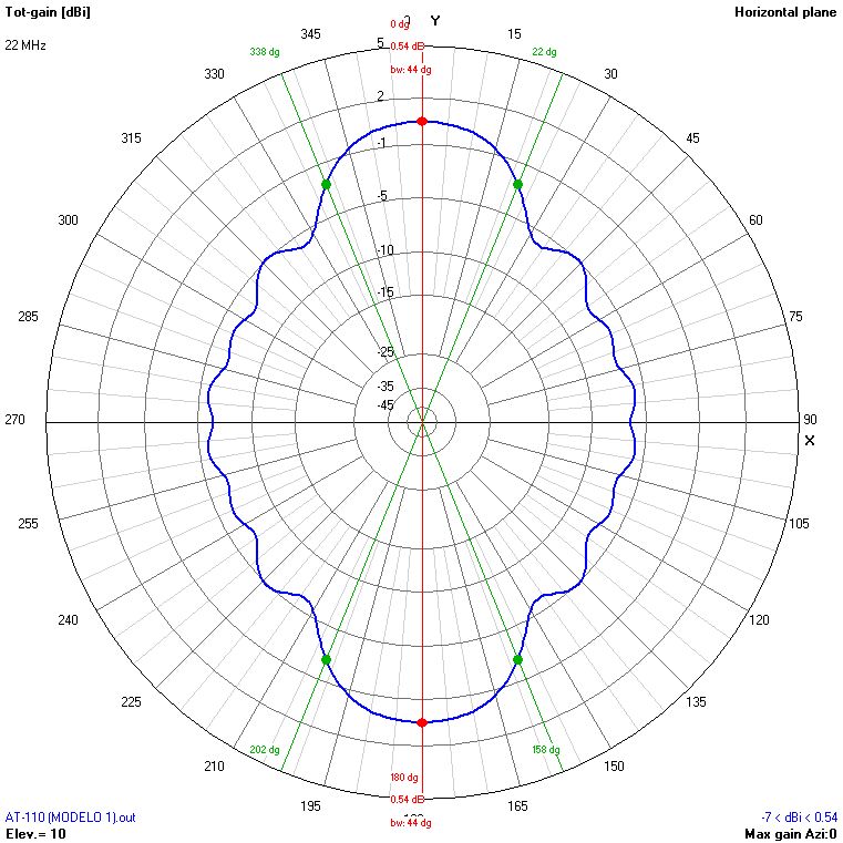
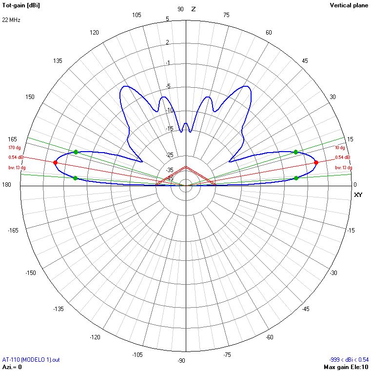
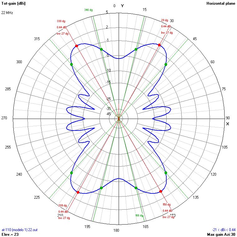
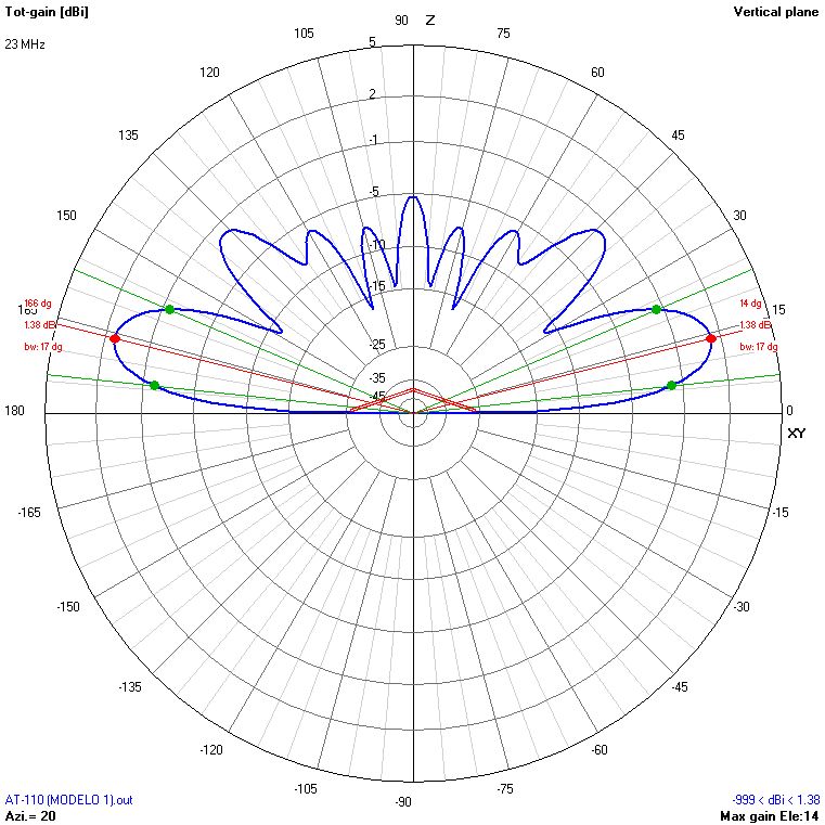
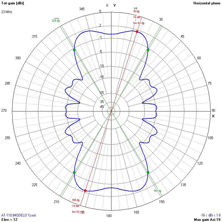
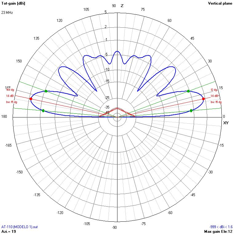
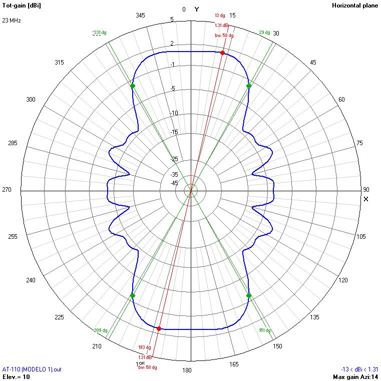
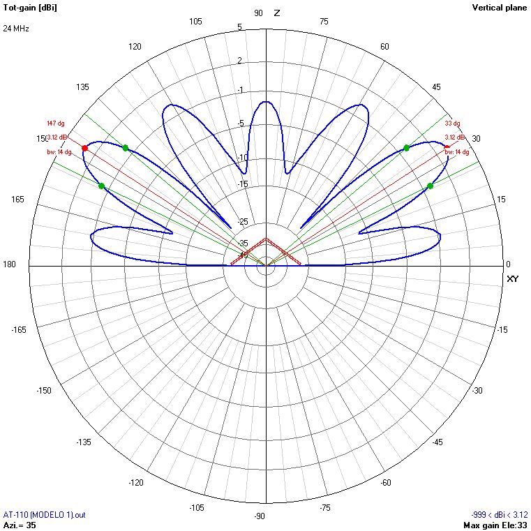
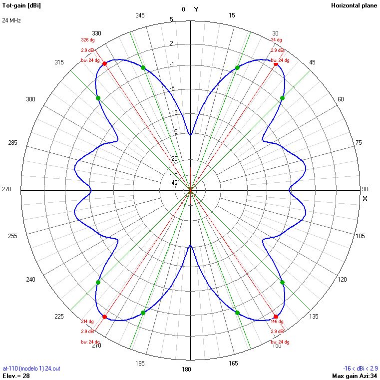
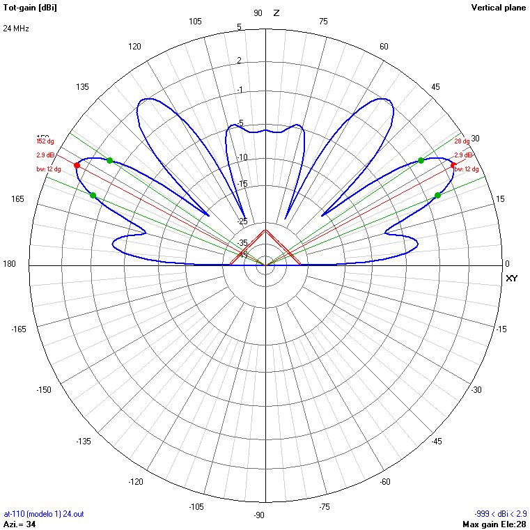
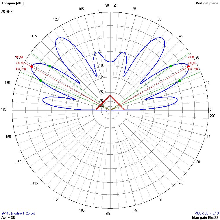
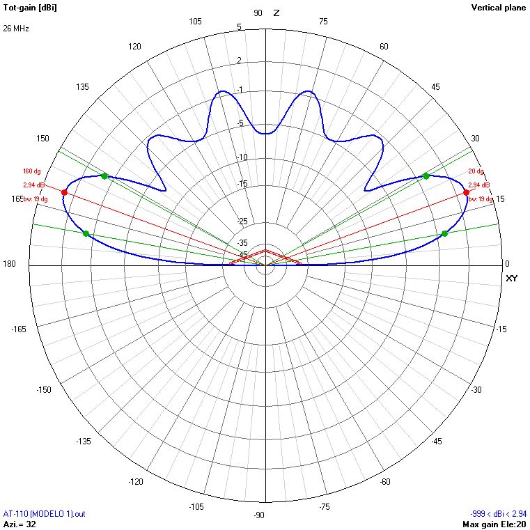
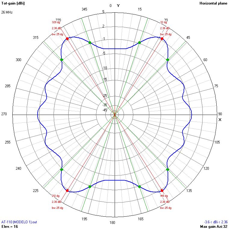
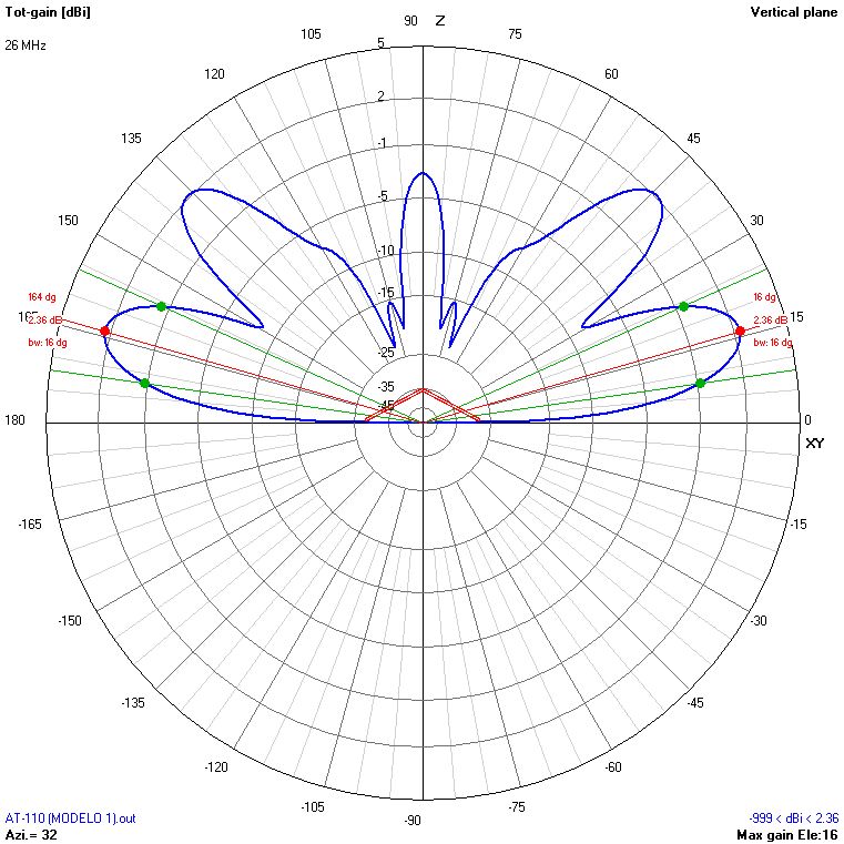
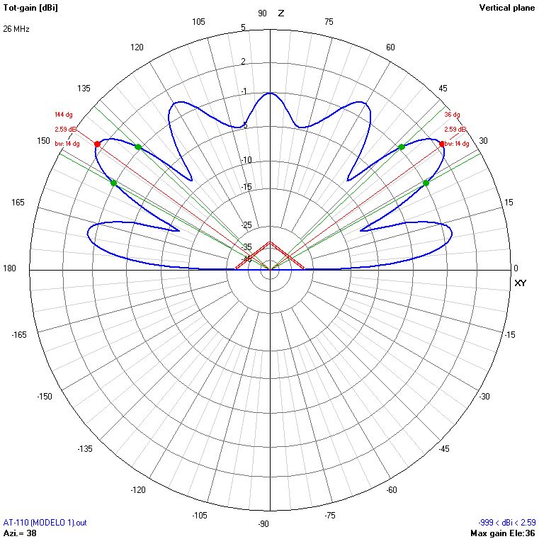
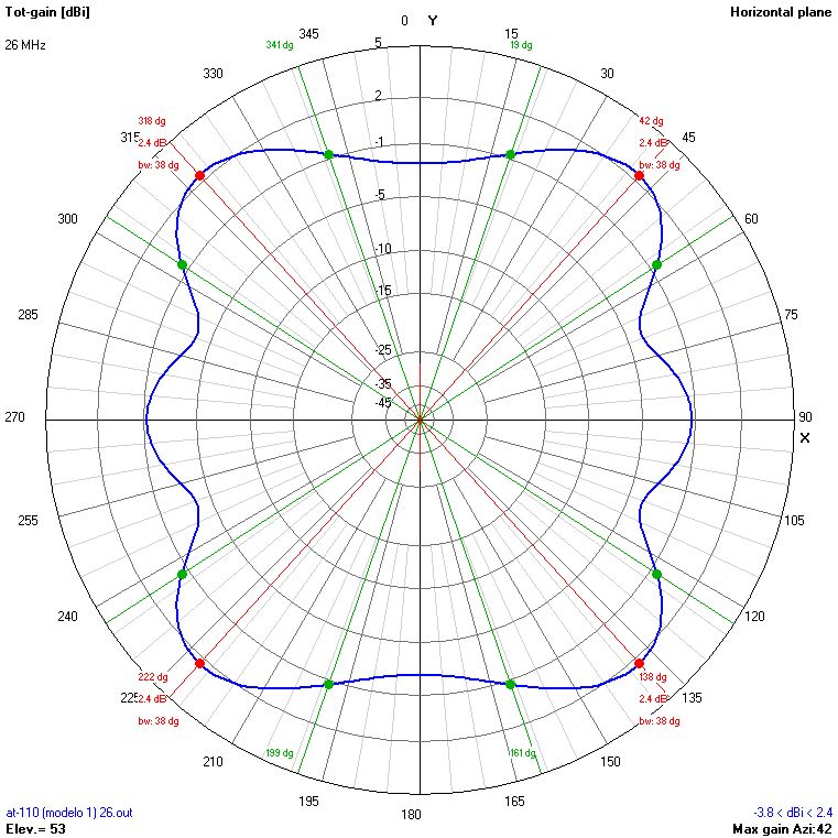
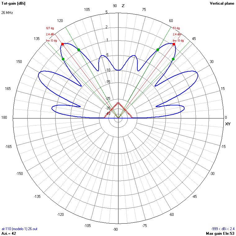
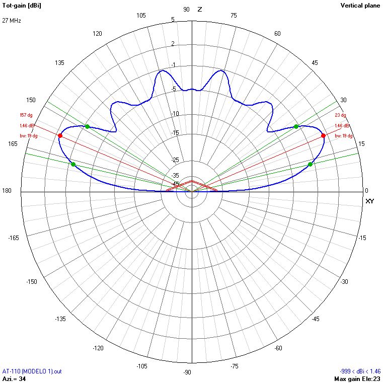
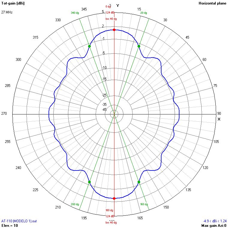
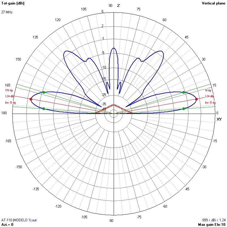
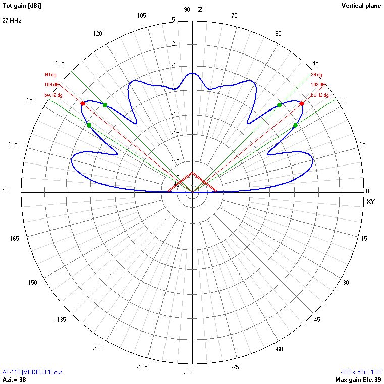
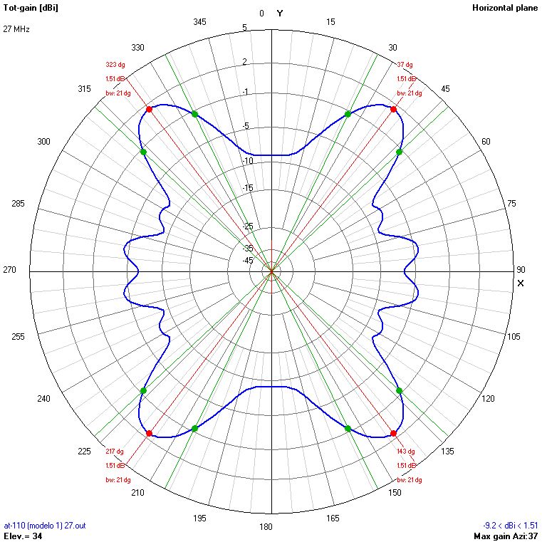
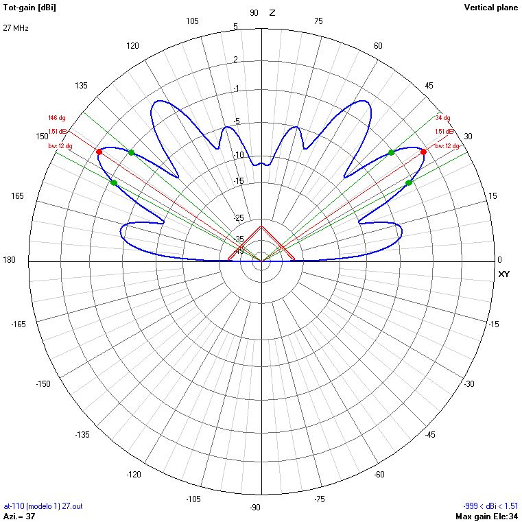
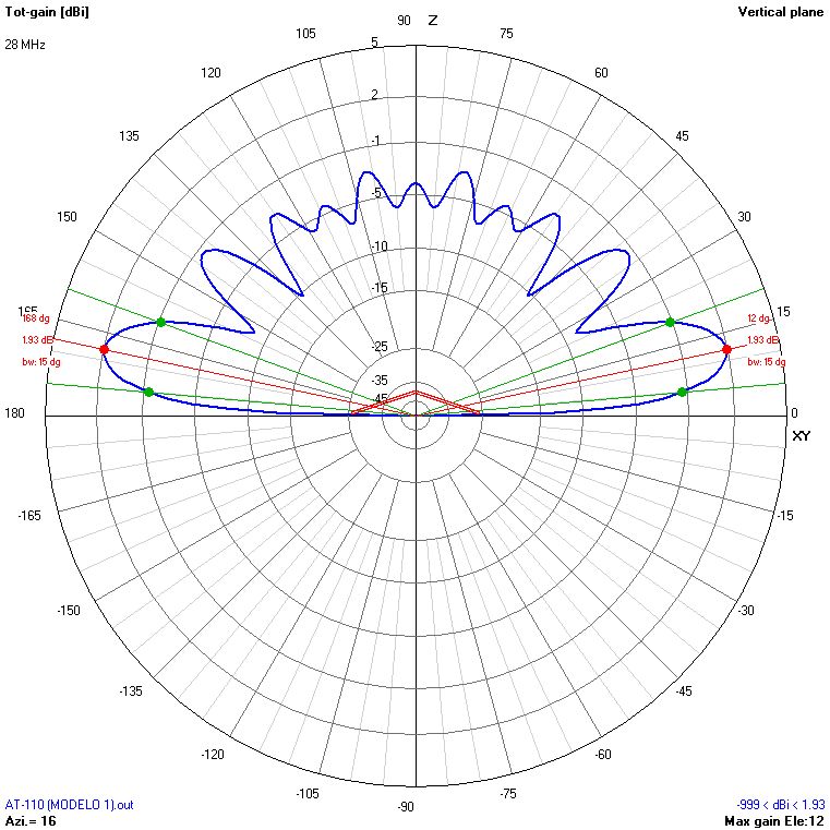
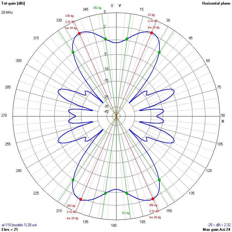
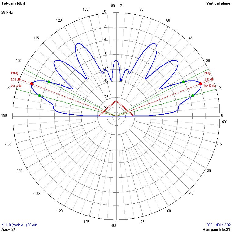
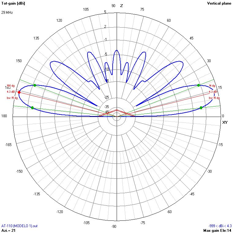
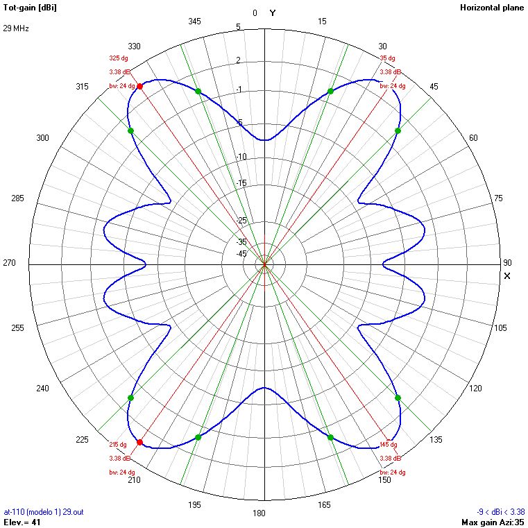
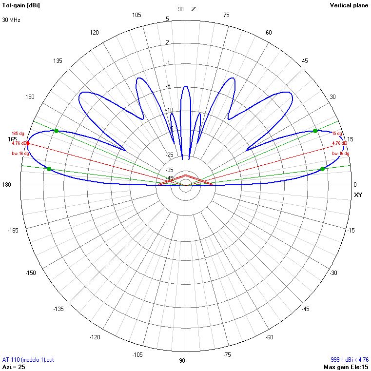
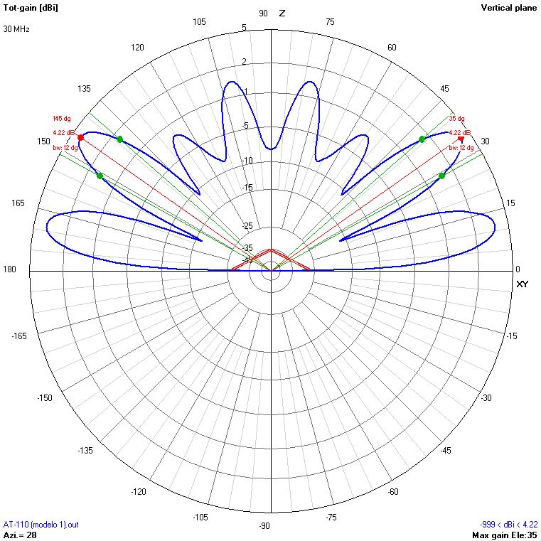
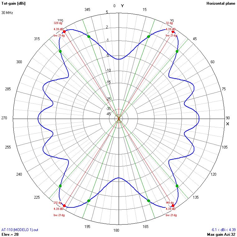
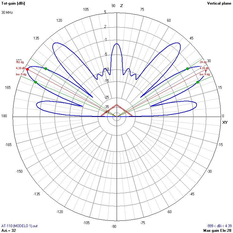
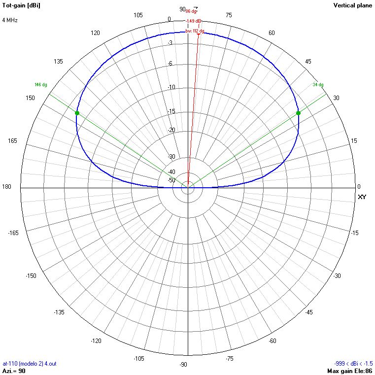
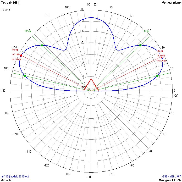
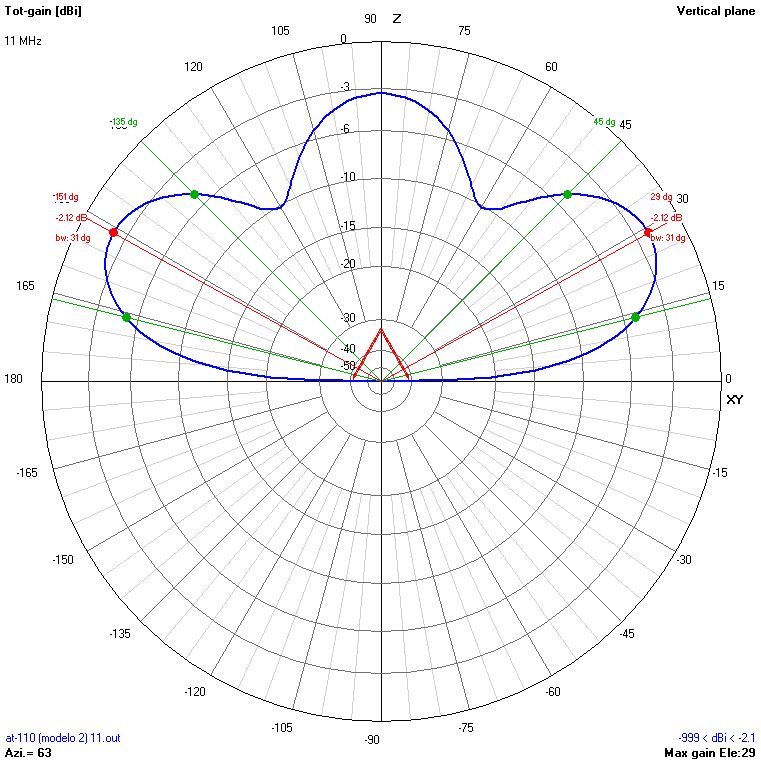
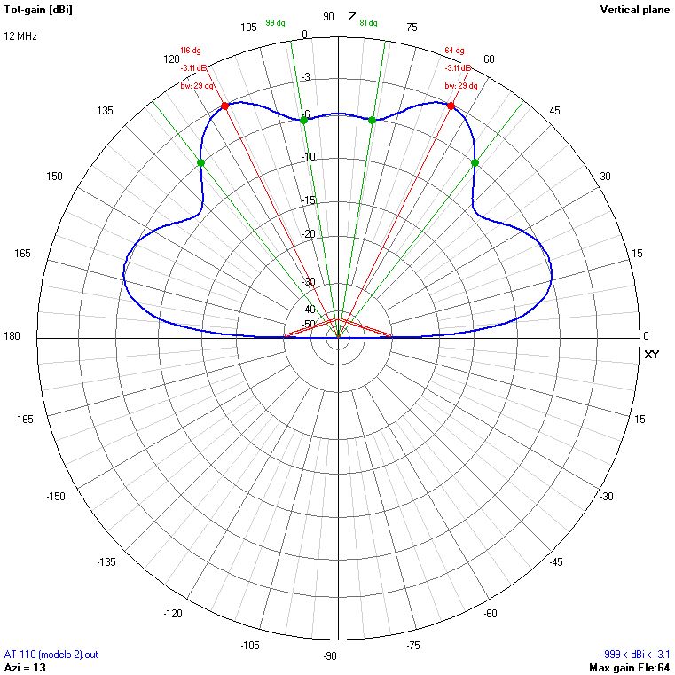
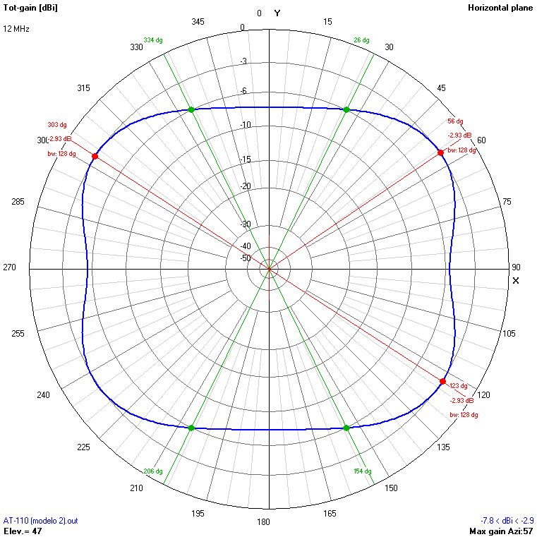
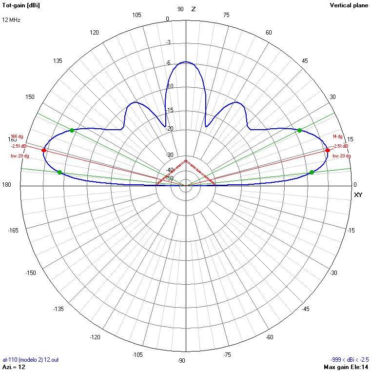
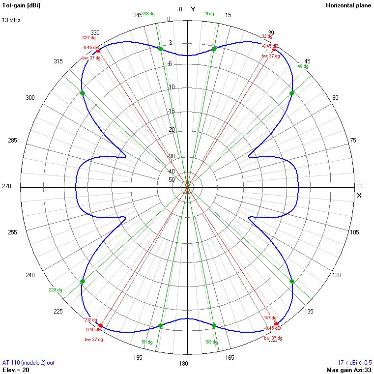
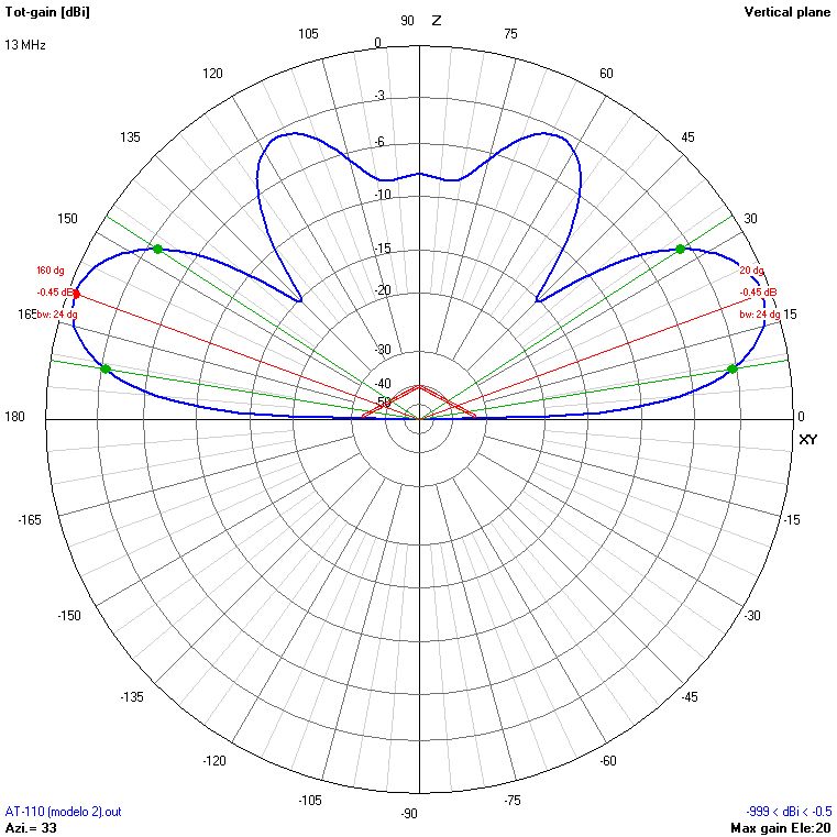
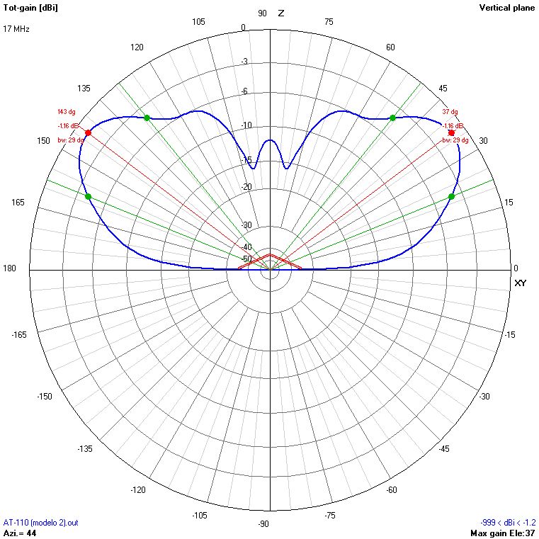
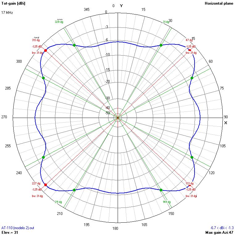
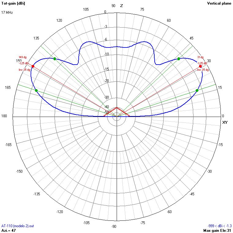
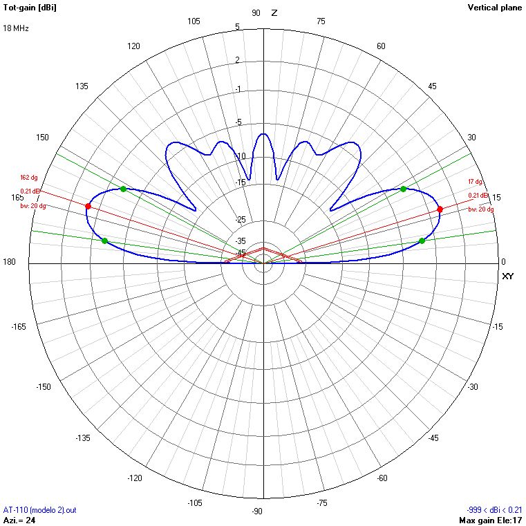
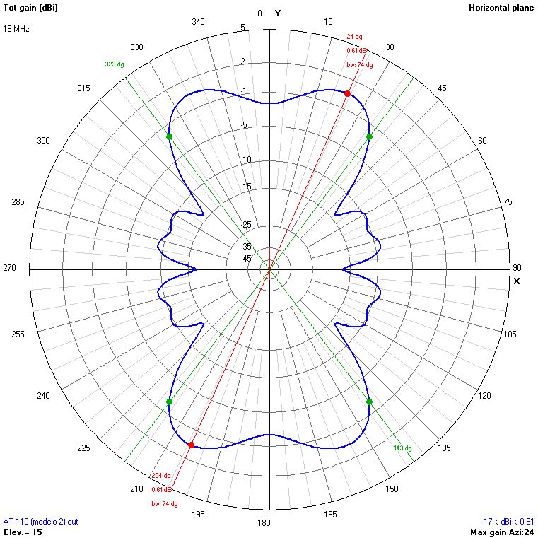
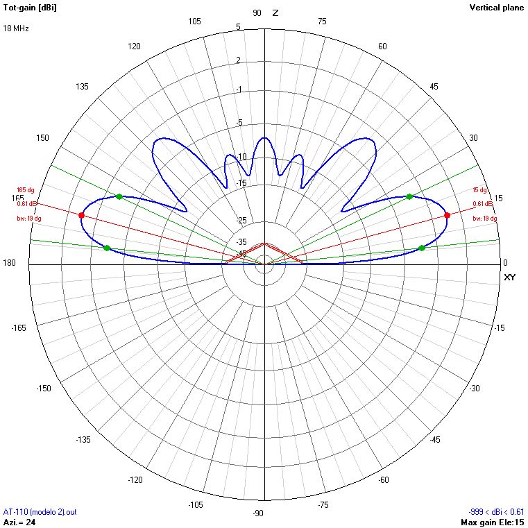
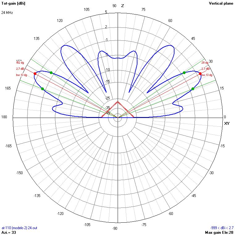
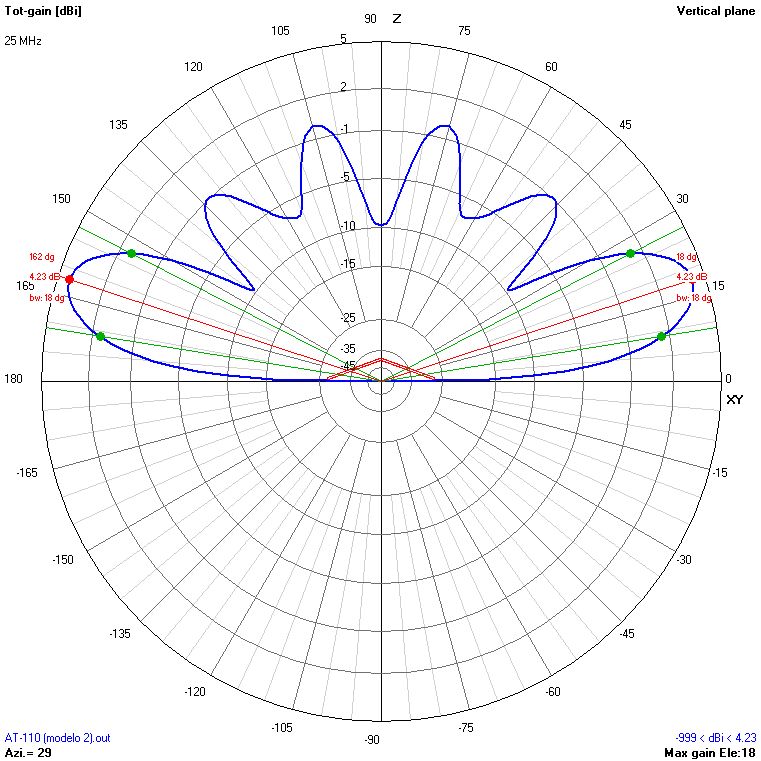
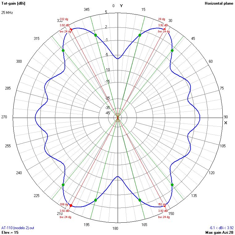
In this section, the results of the simulations of the model 1 are shown (see section 2.1), consisting of radiation patterns for frequencies between 2 MHz and 30 MHz at 1 MHz intervals and for masts of 9, 12, 15 and 18 m. The antenna is installed in inverted-vee configuration with the tips at 0,5 metres over ground.
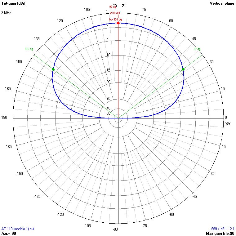
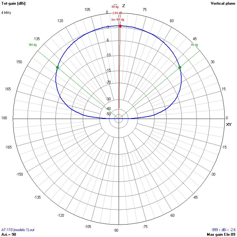
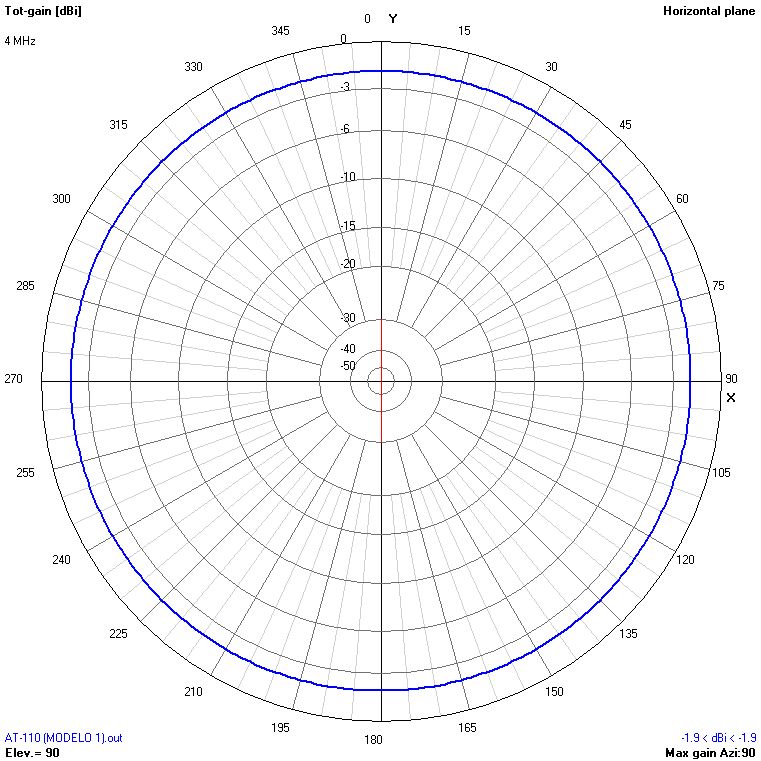
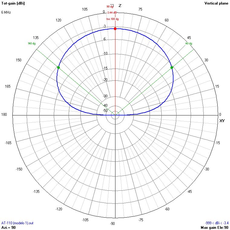
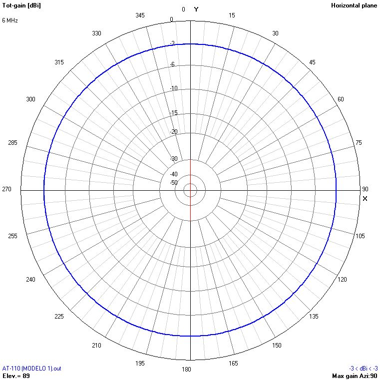
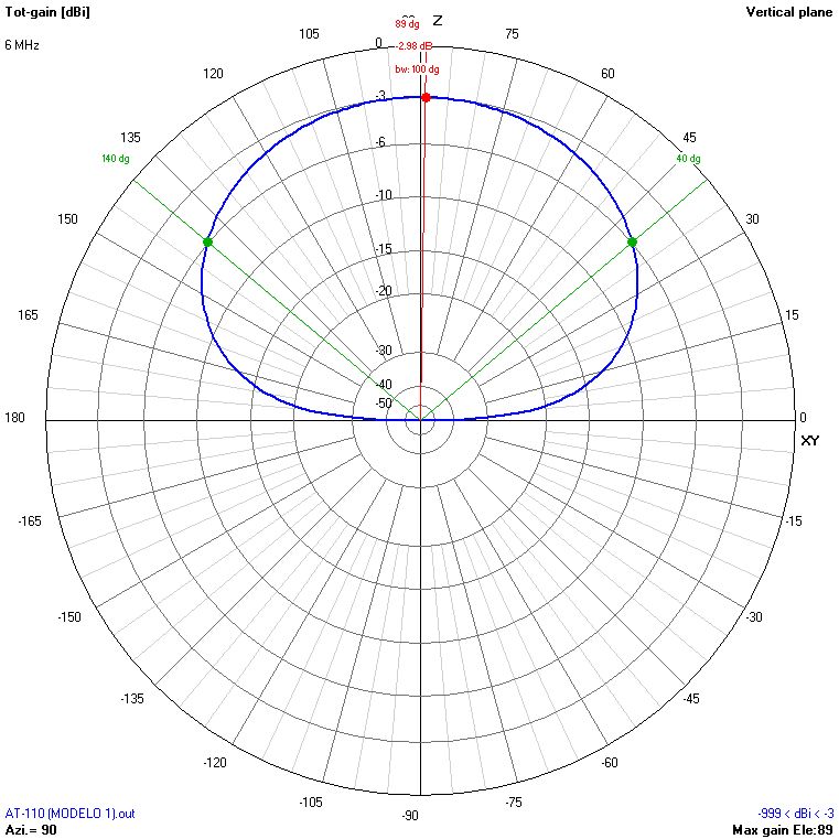
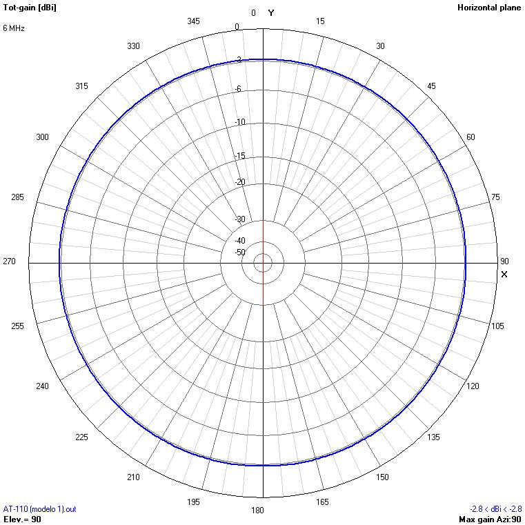
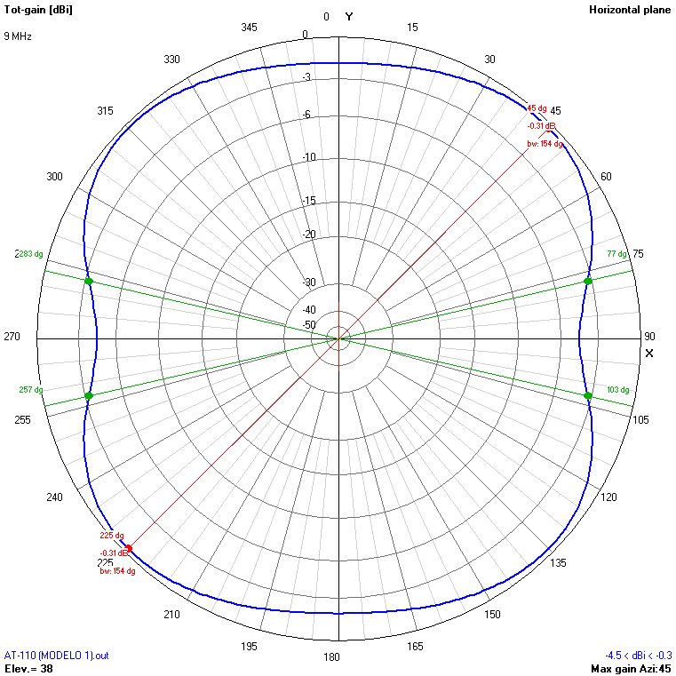
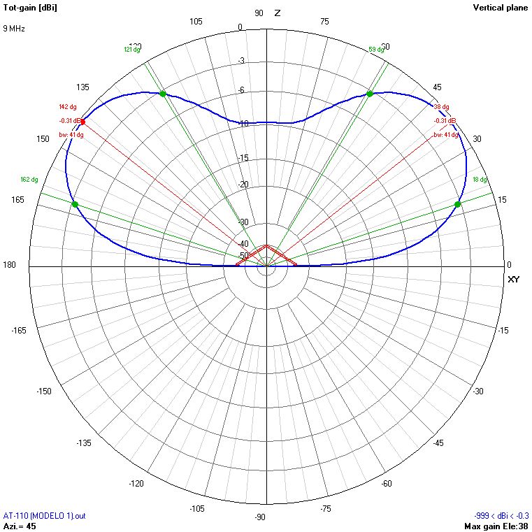
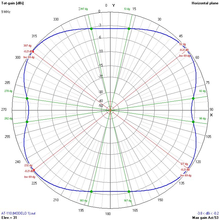
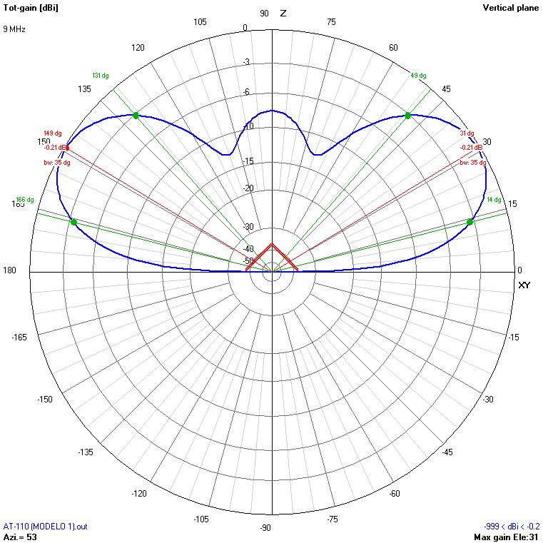
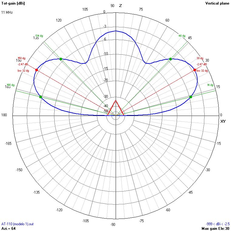
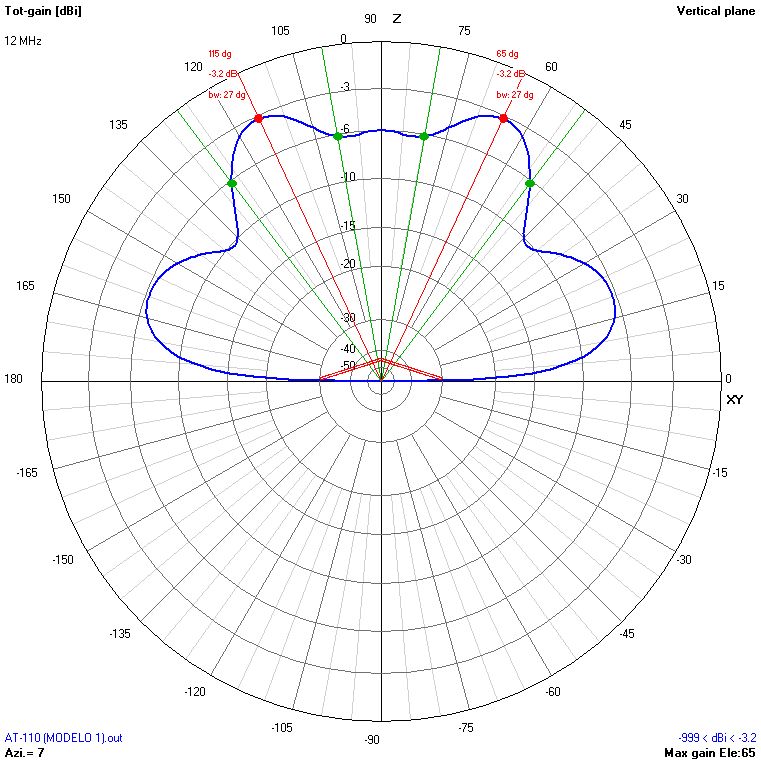
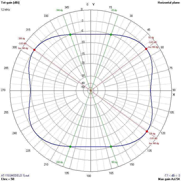
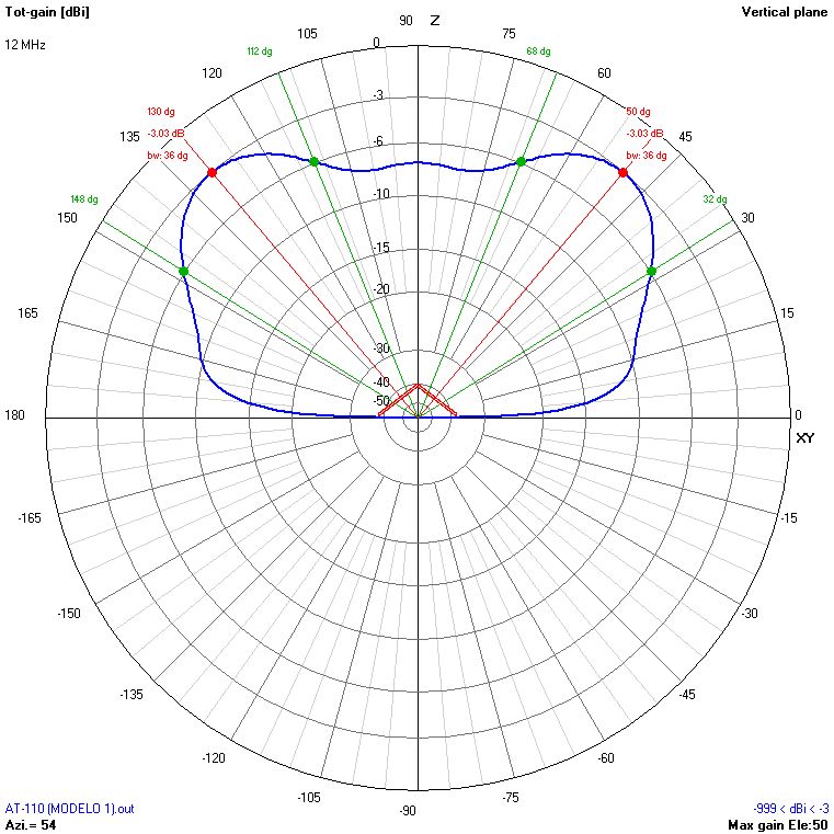
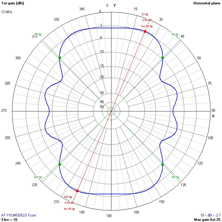
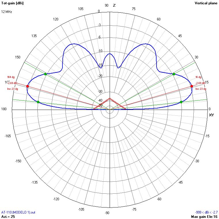
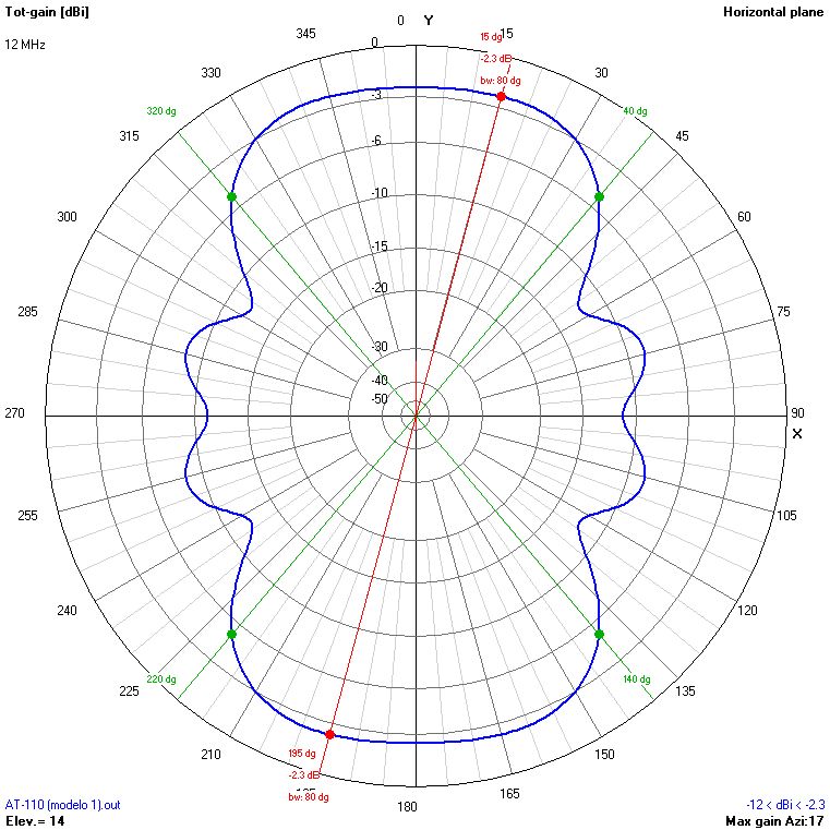
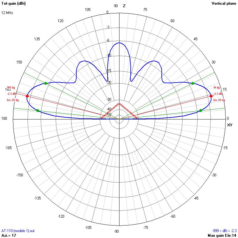
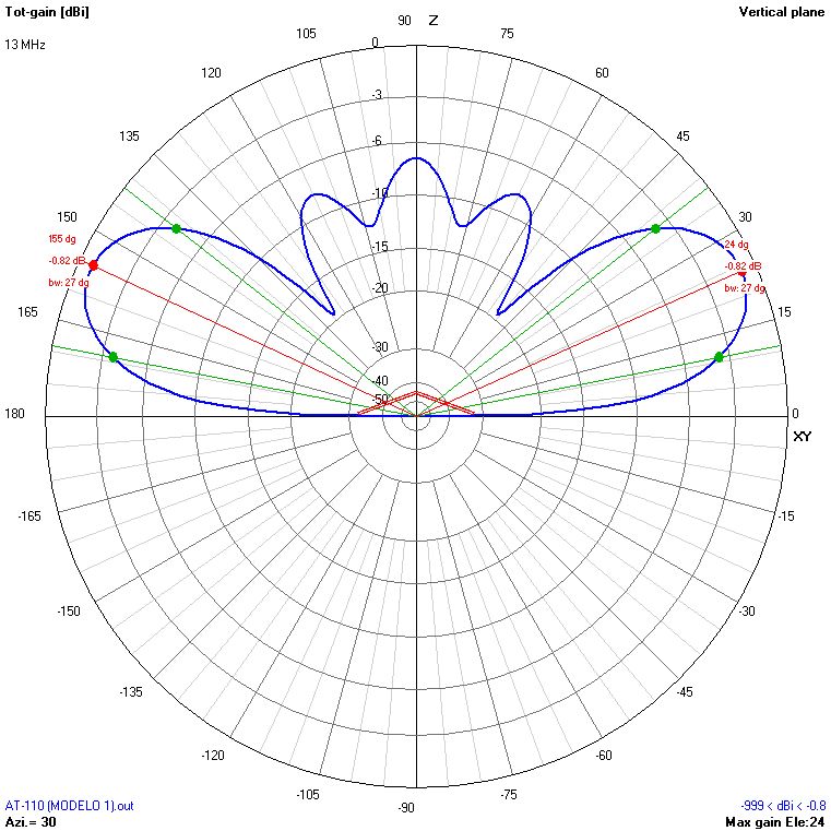
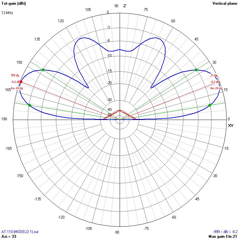
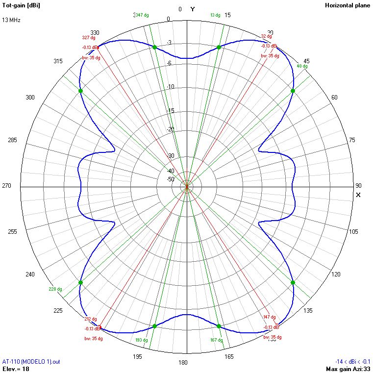
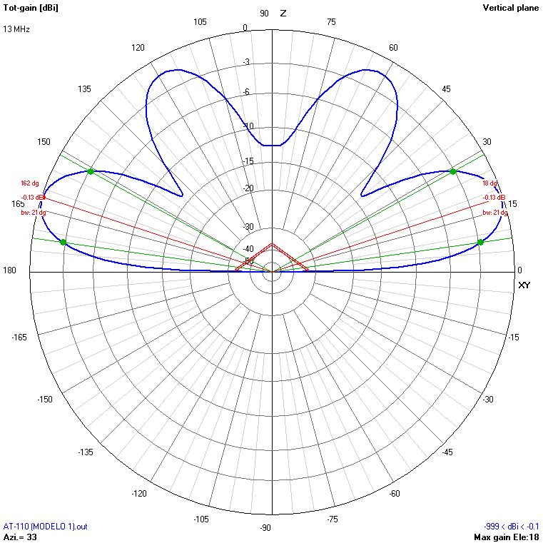
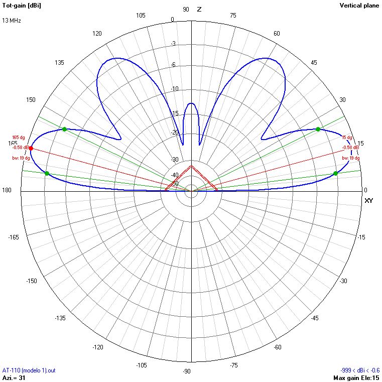
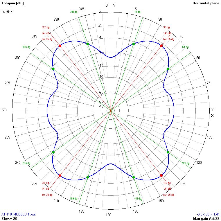
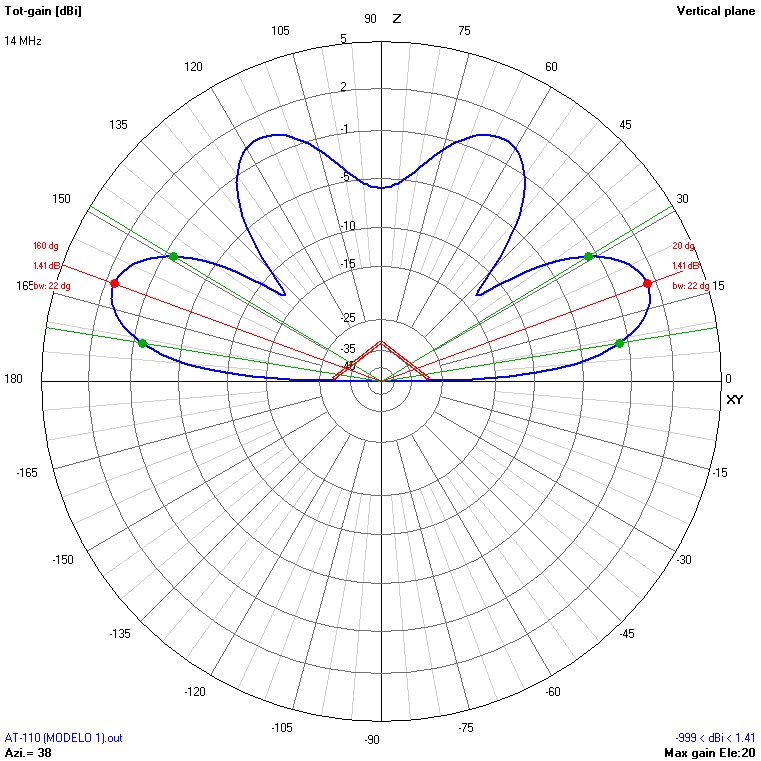
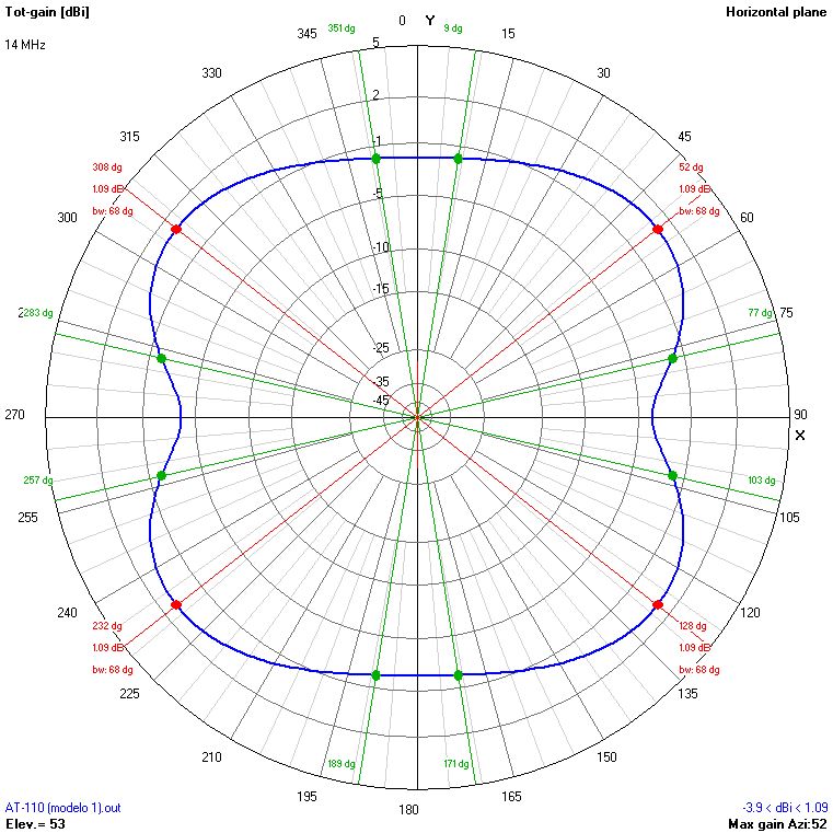
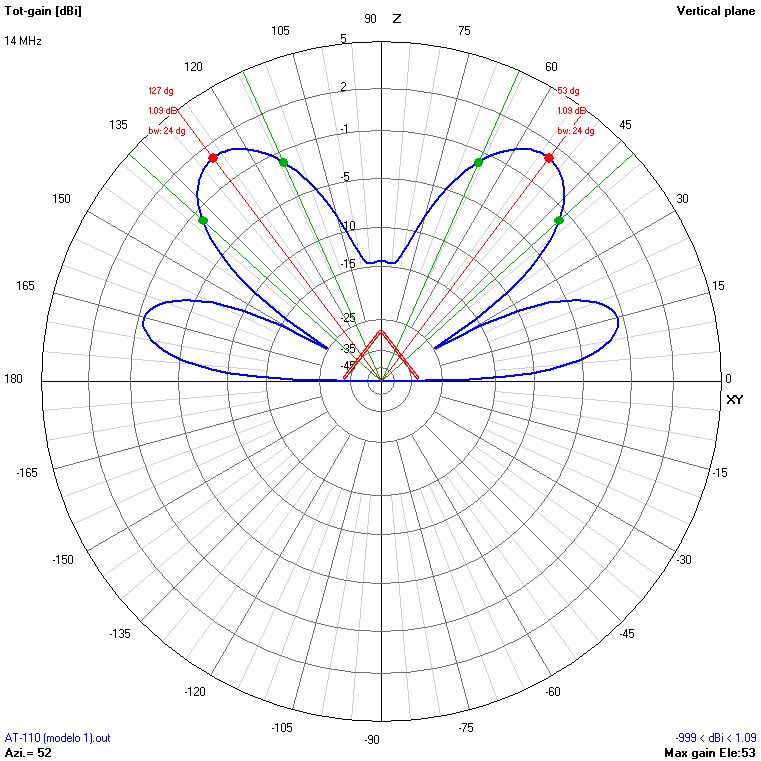
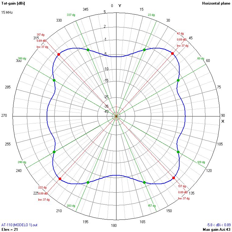
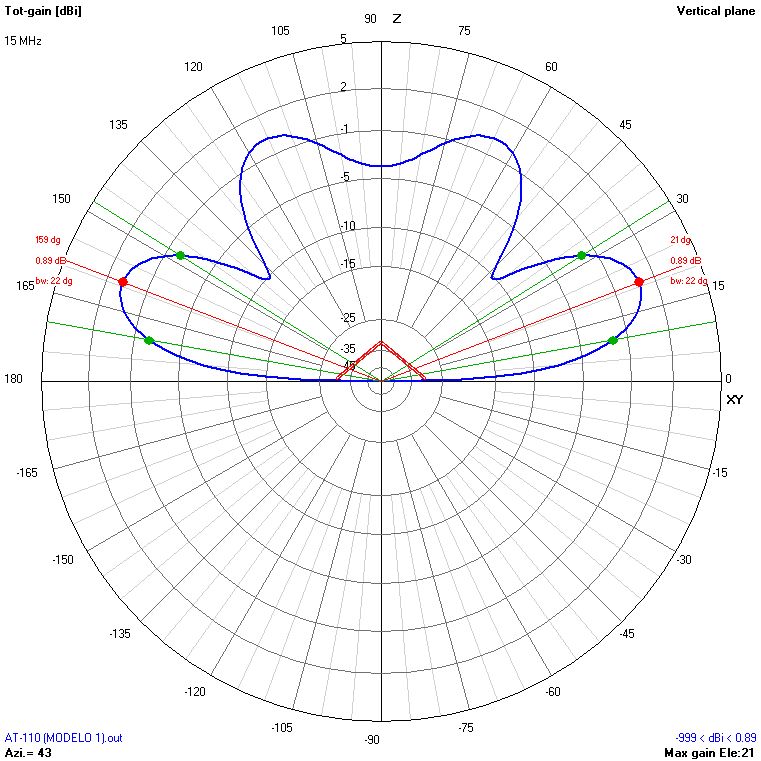
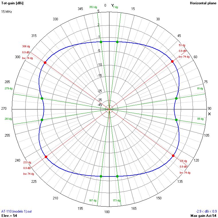
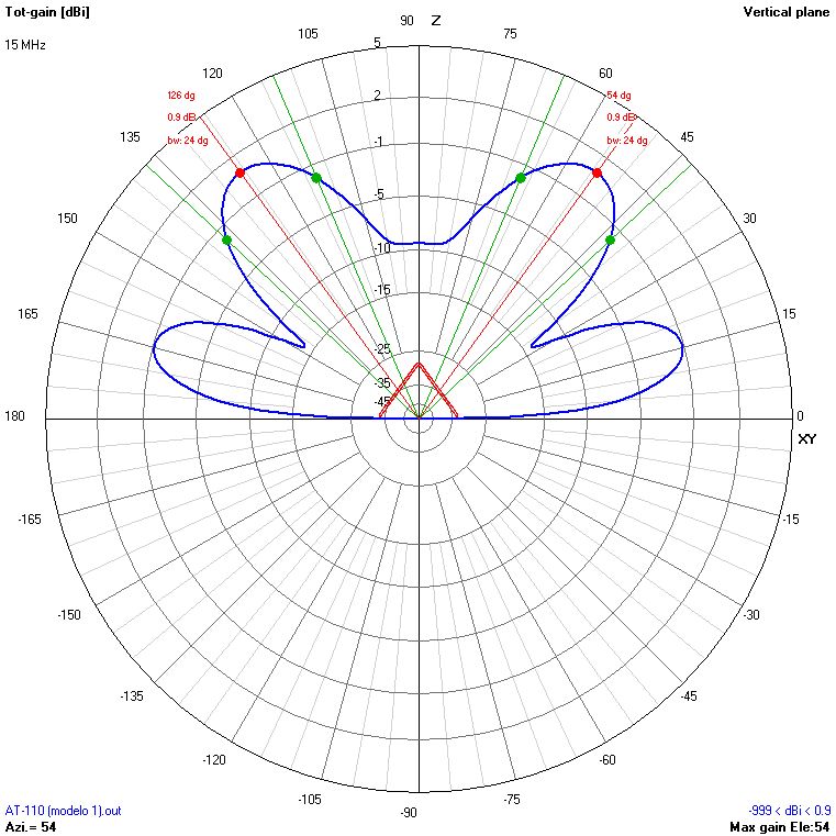
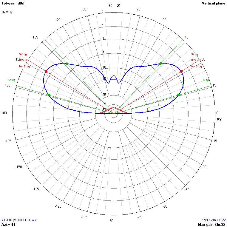
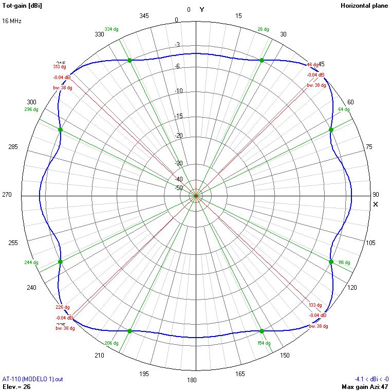
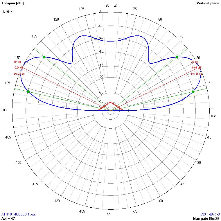
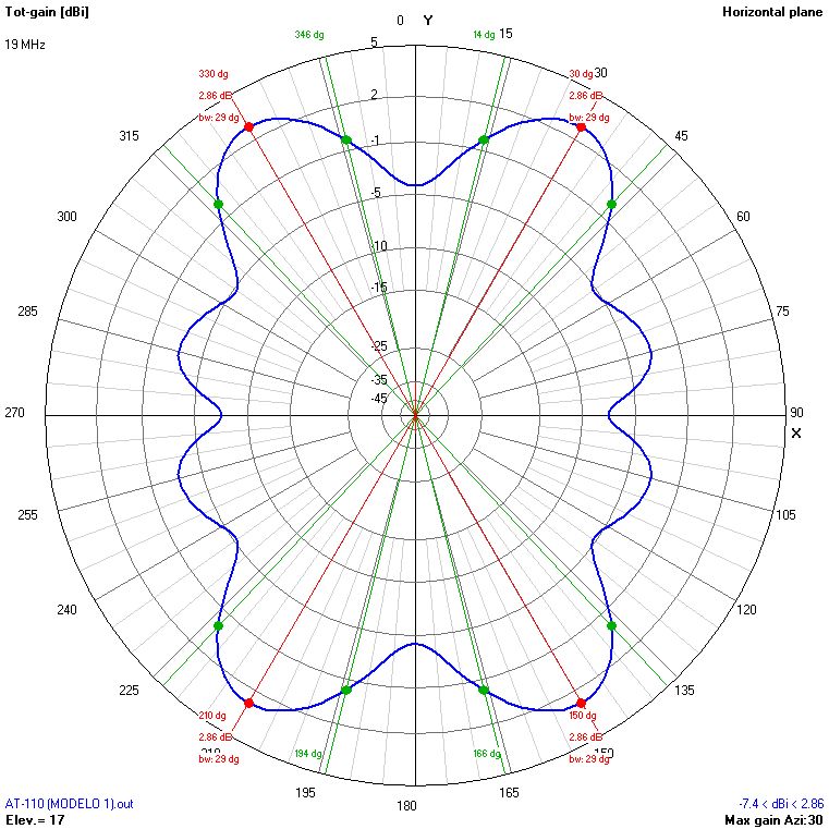
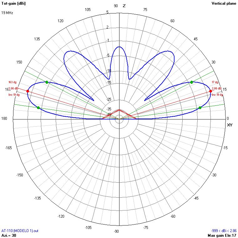
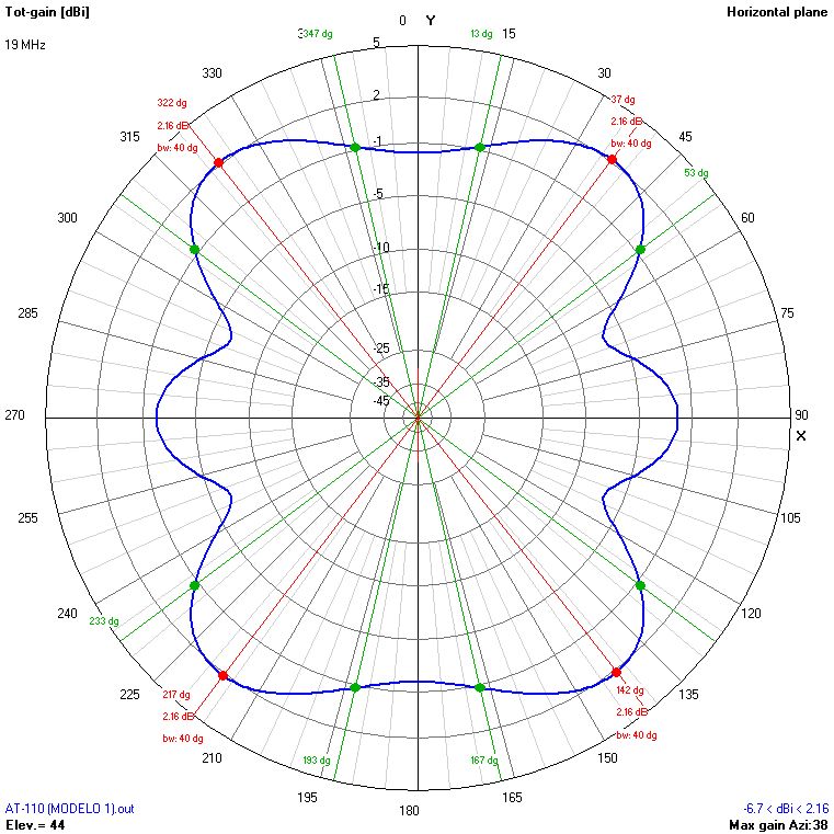
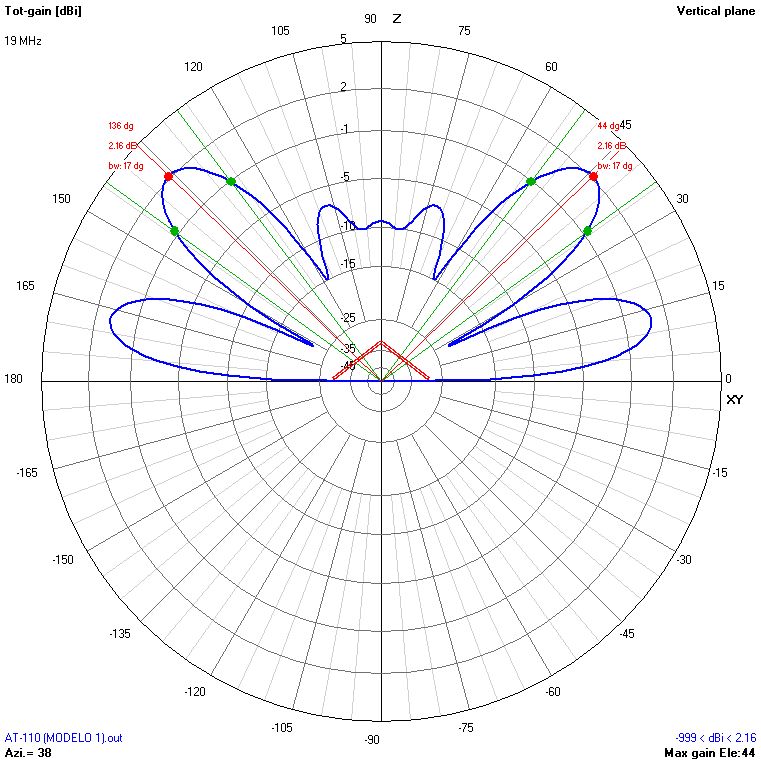
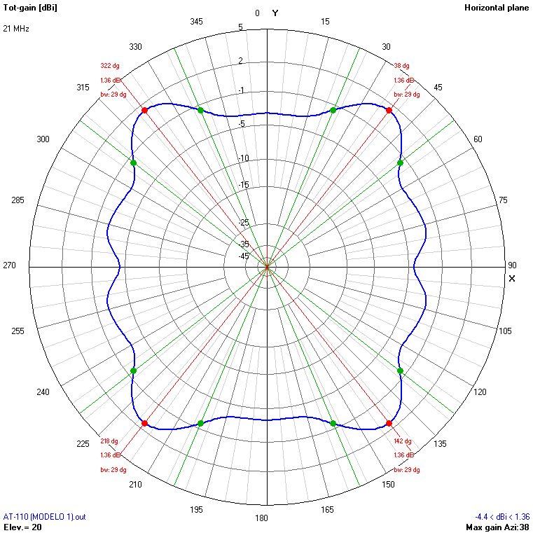
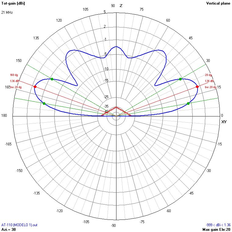
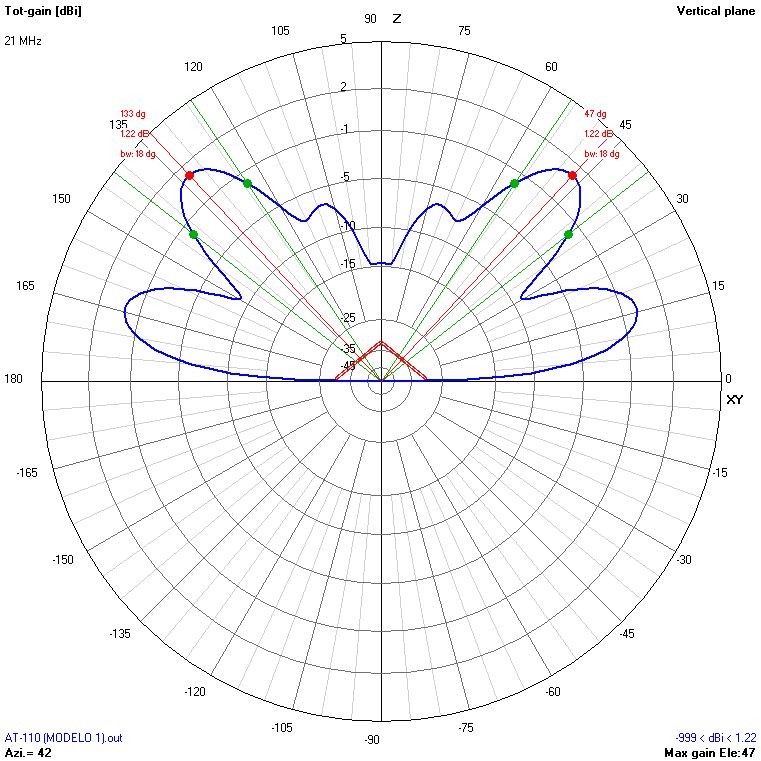
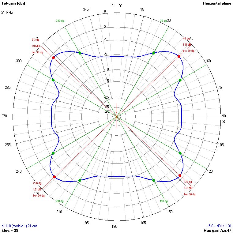
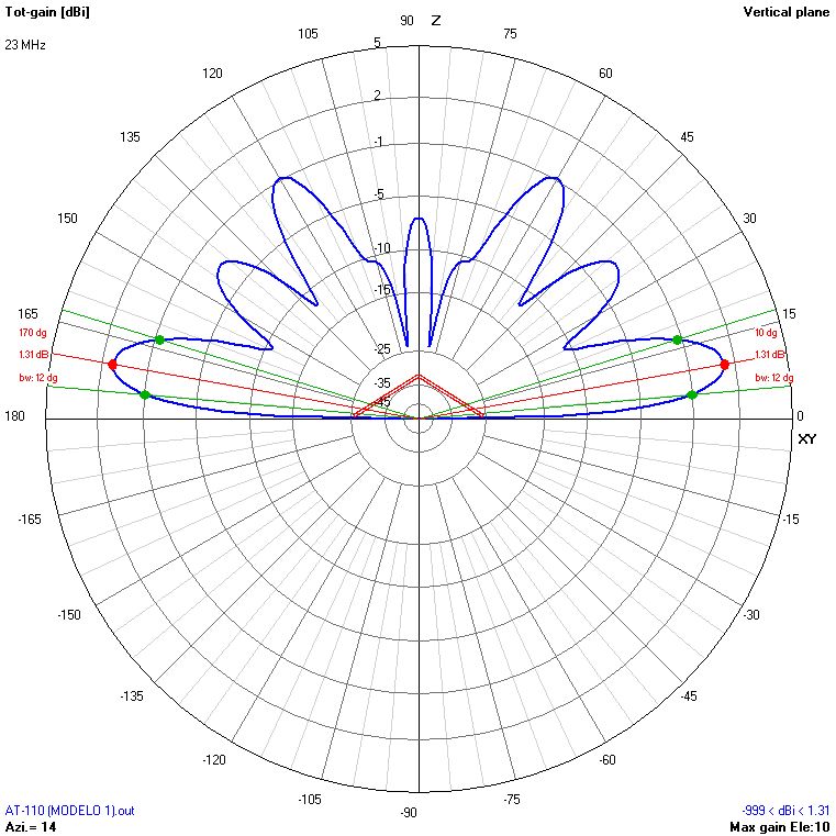
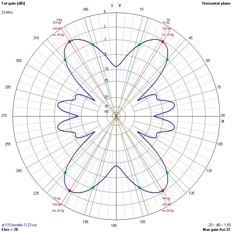
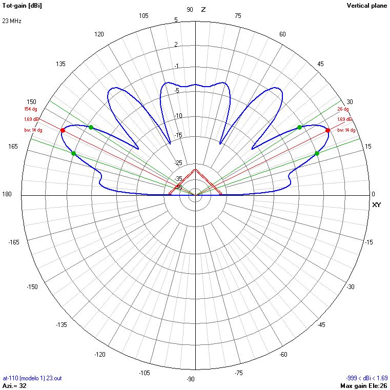
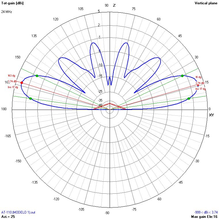
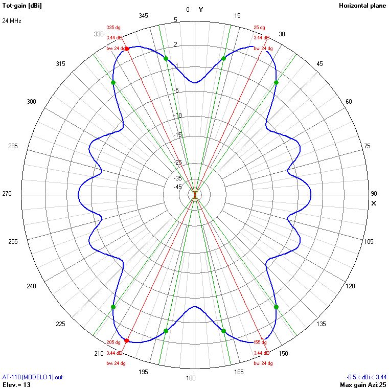
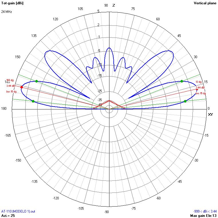
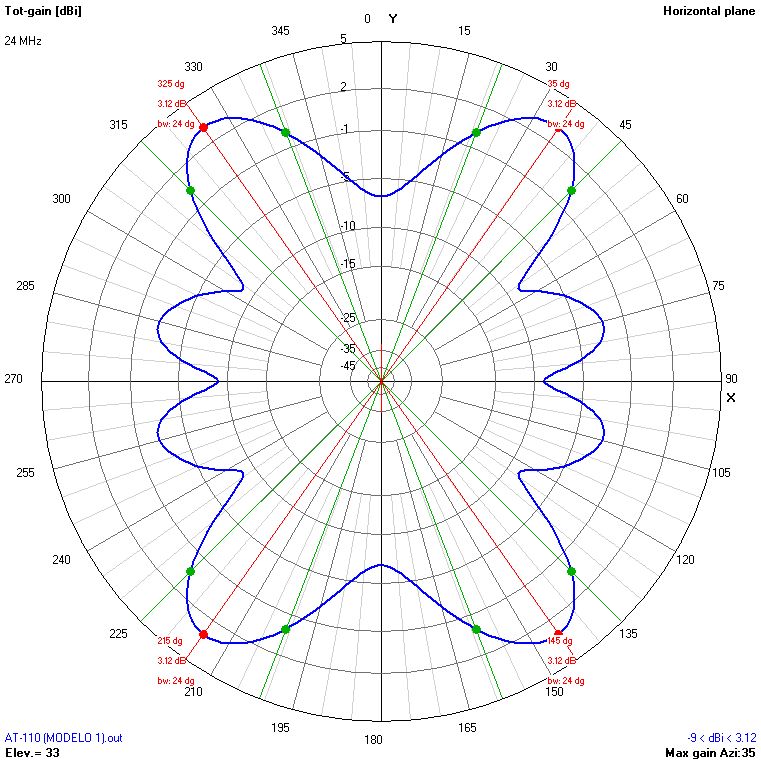
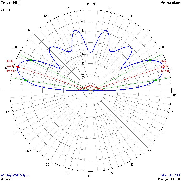
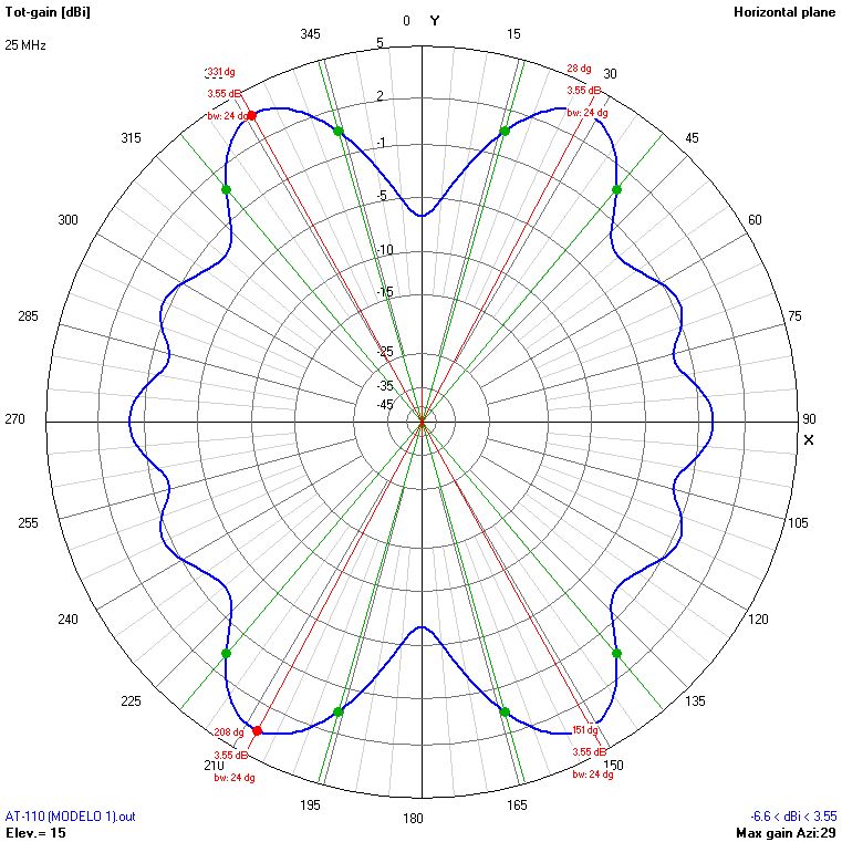
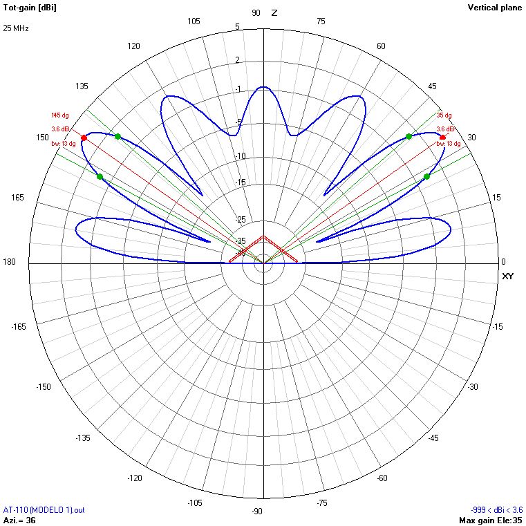
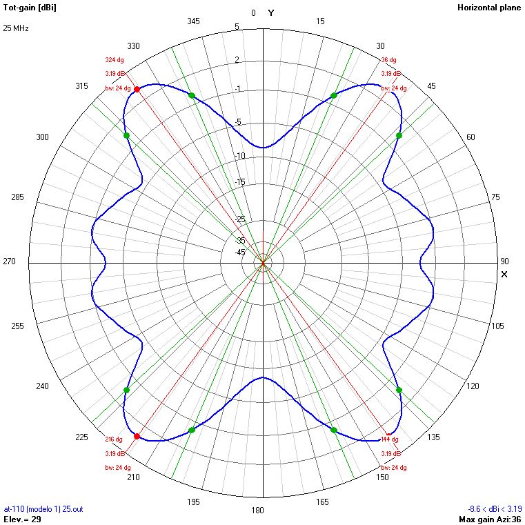
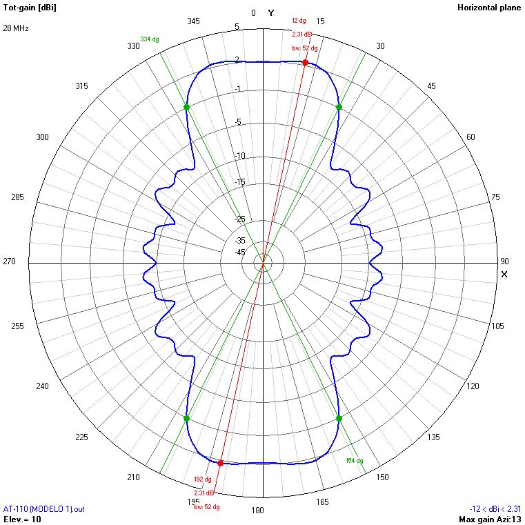
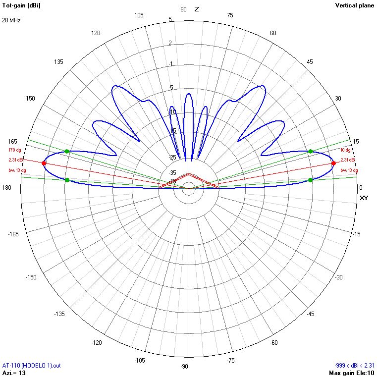
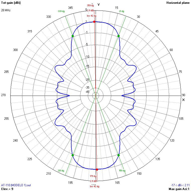
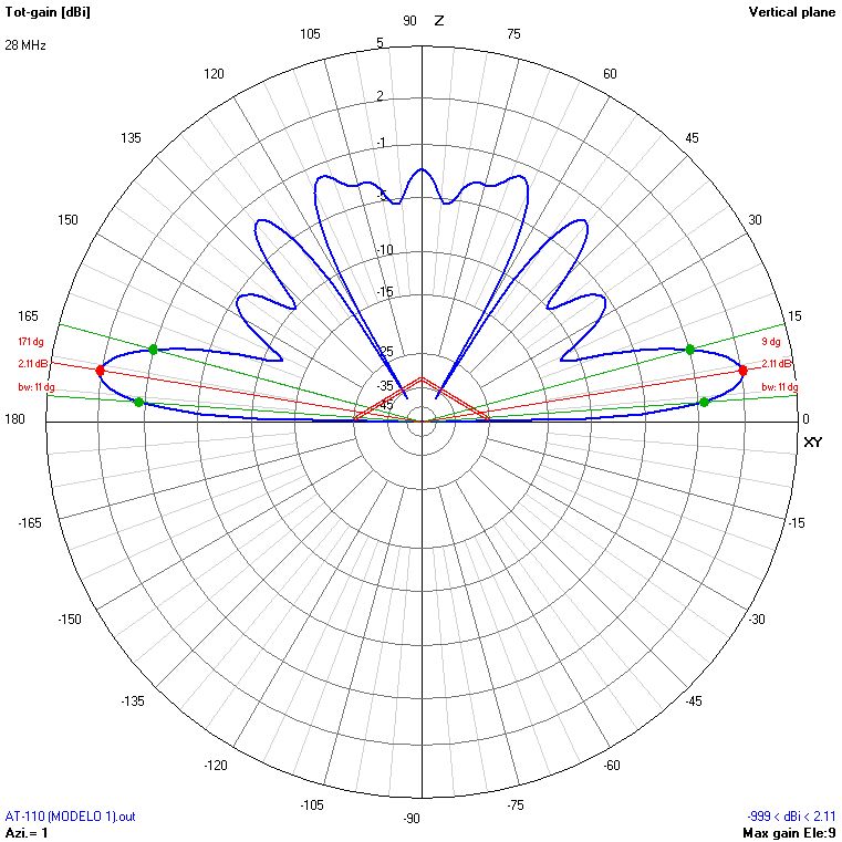
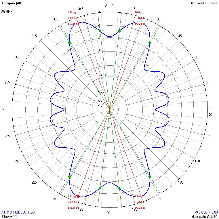
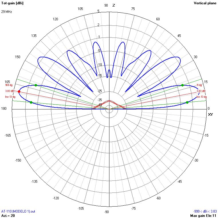
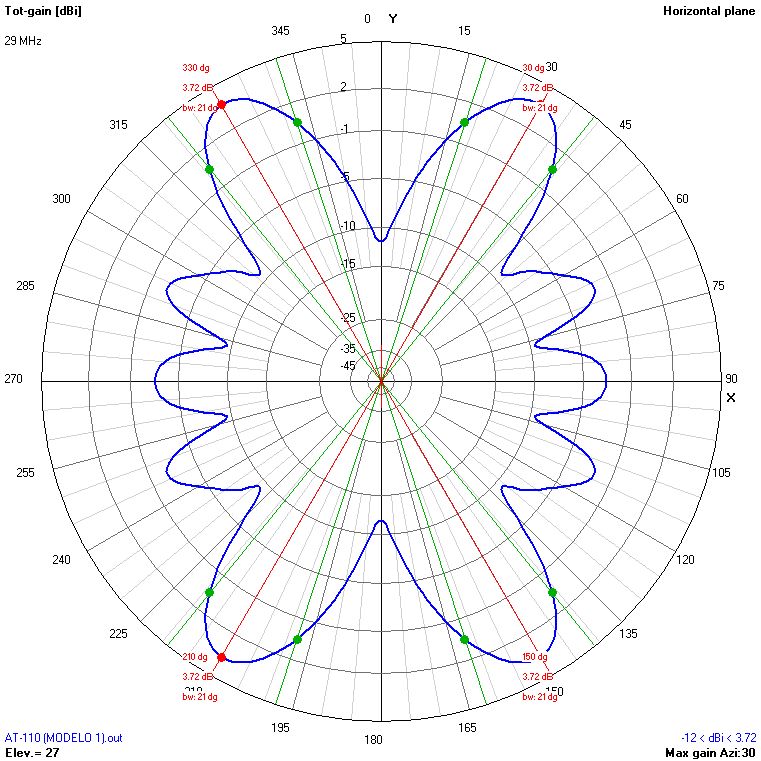
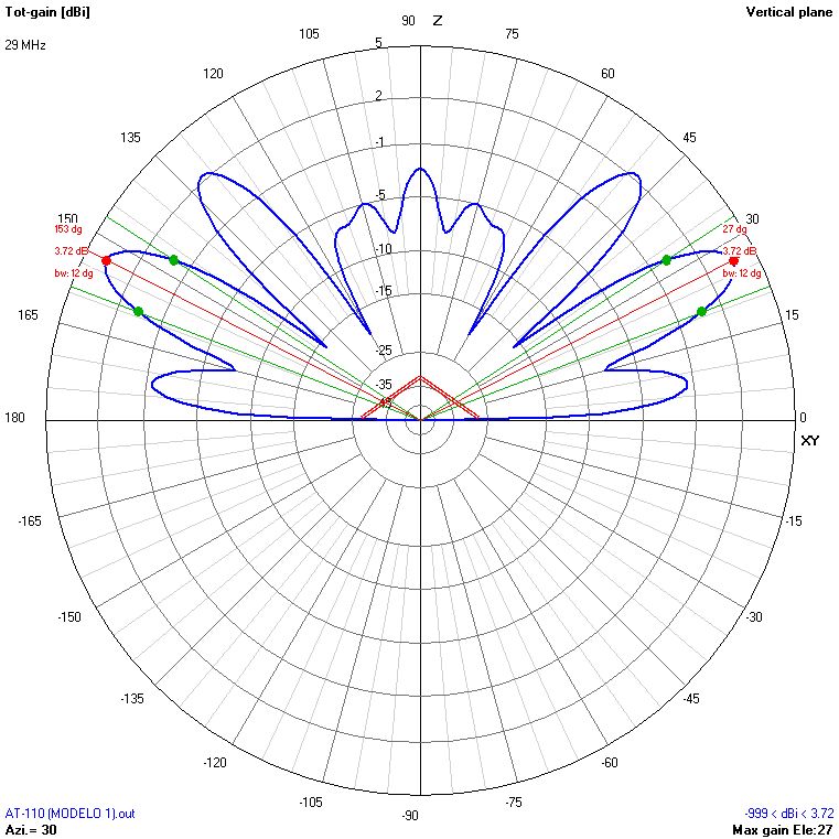
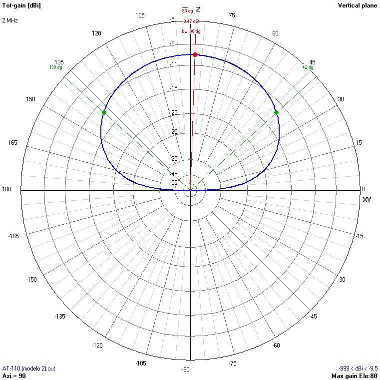
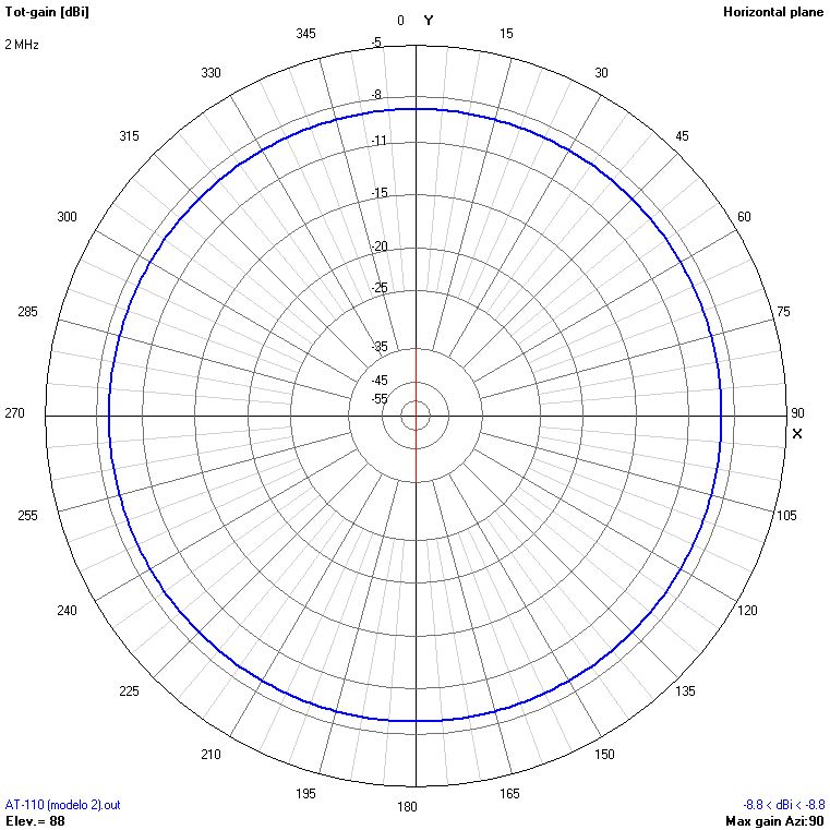
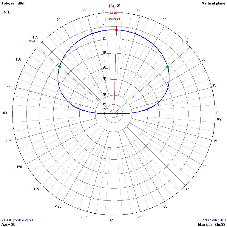
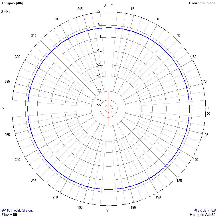
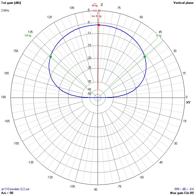
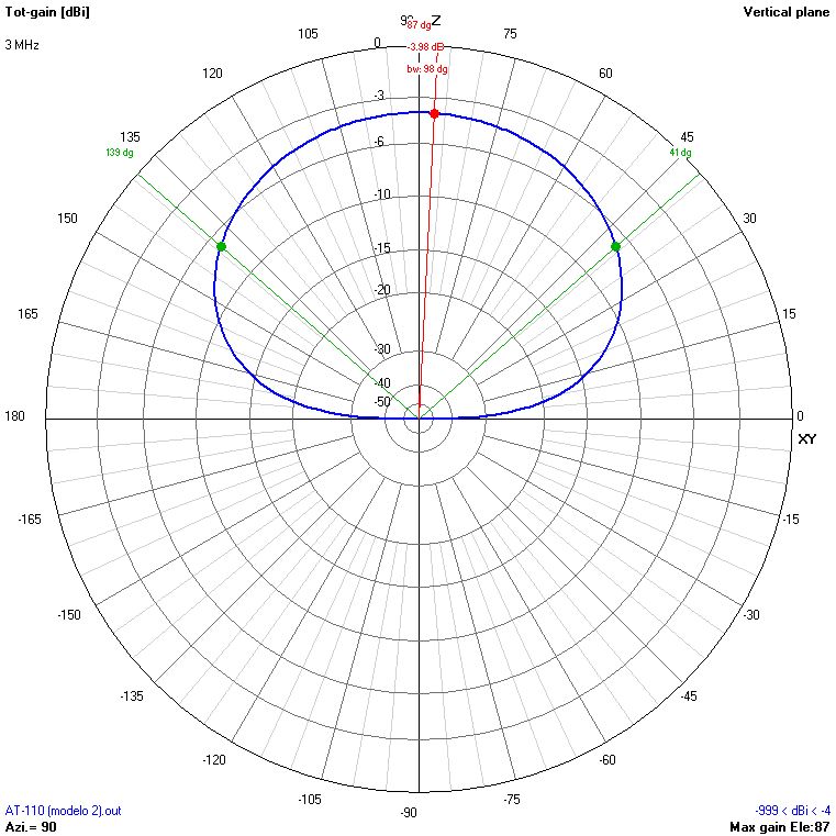
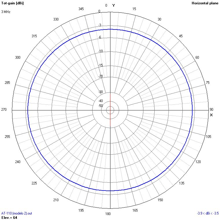
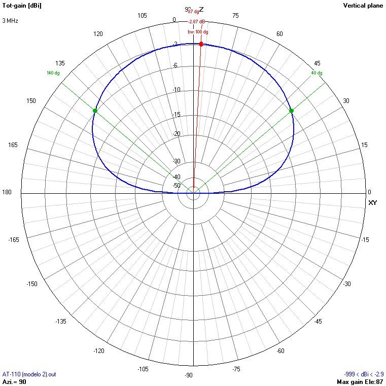
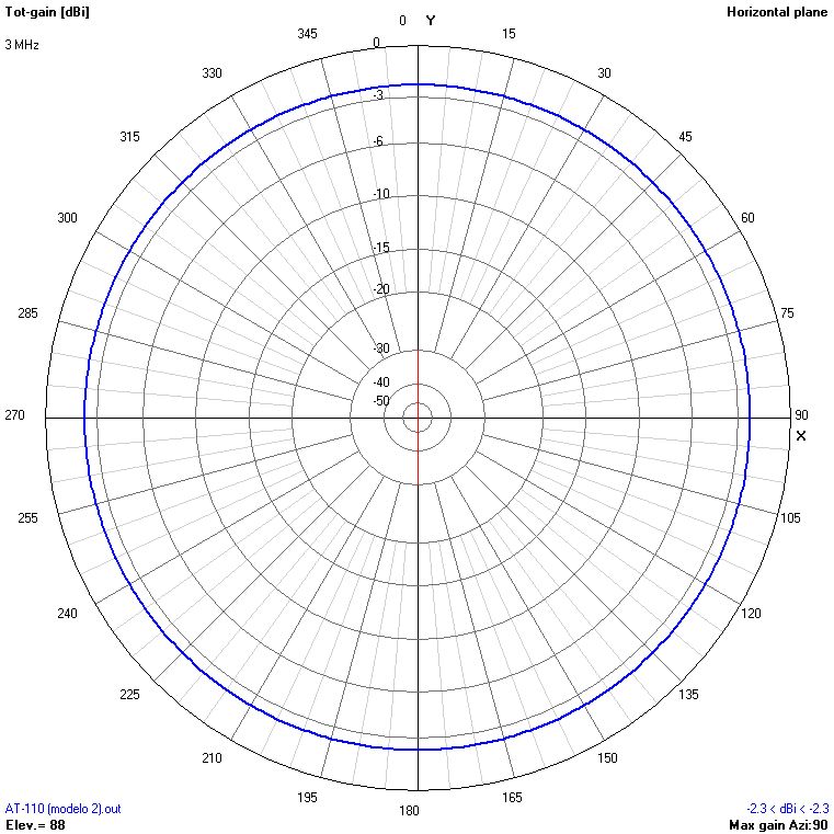
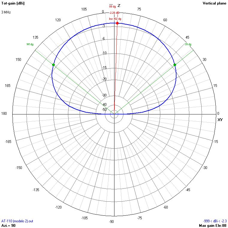
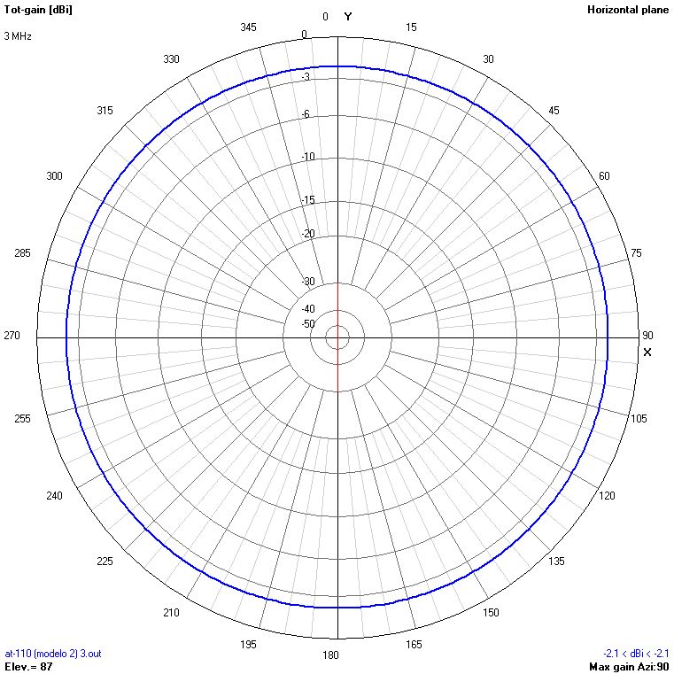
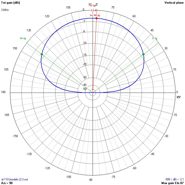
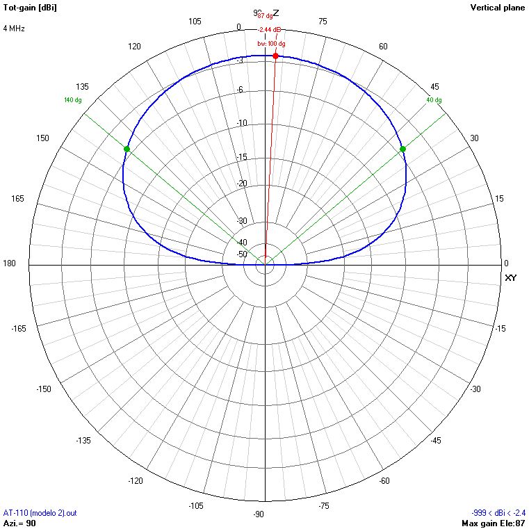
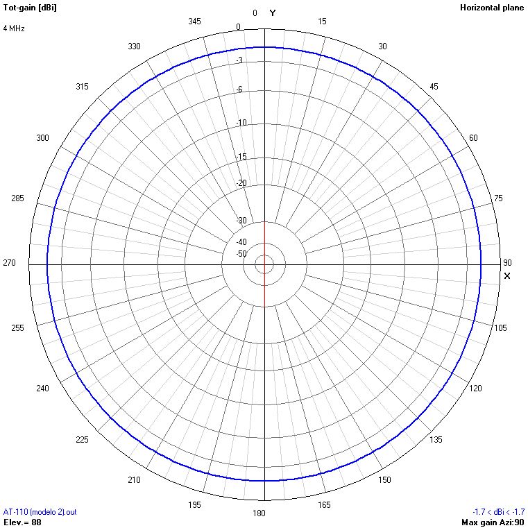
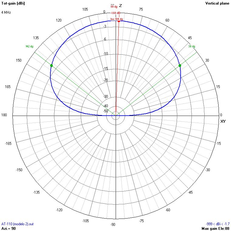
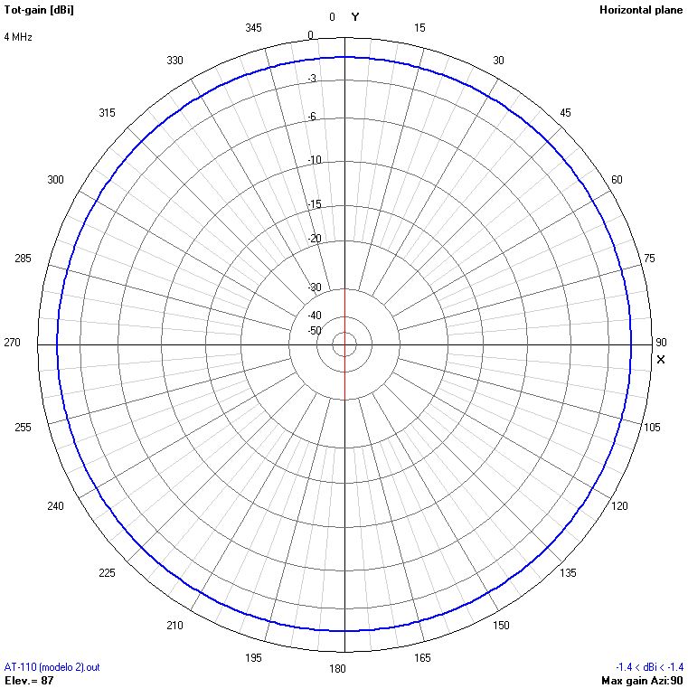
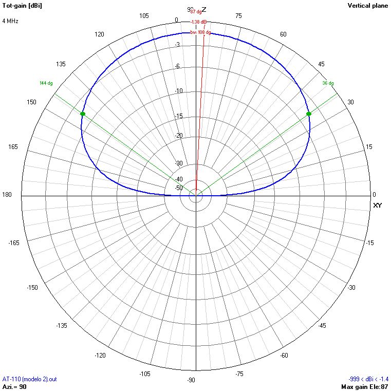
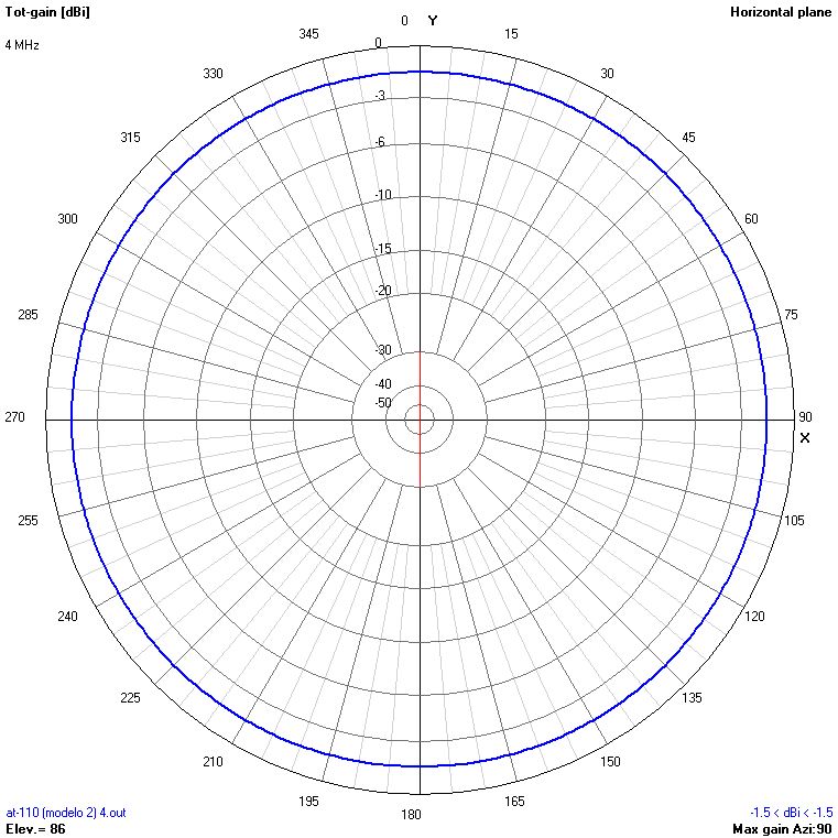
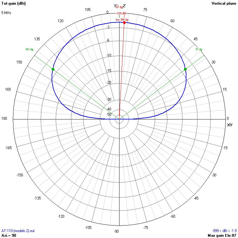
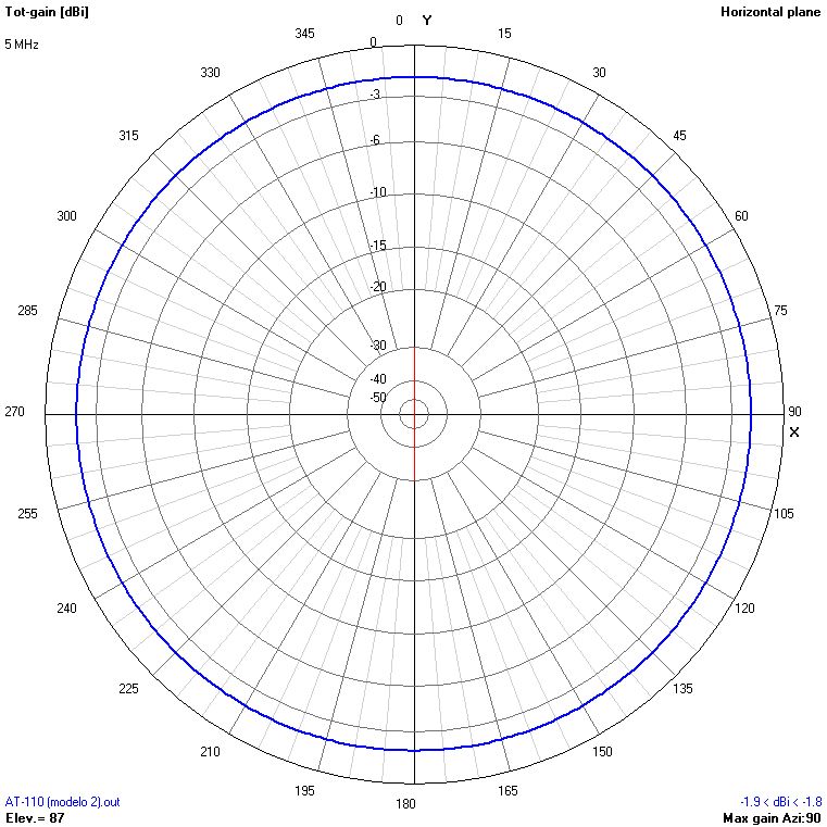
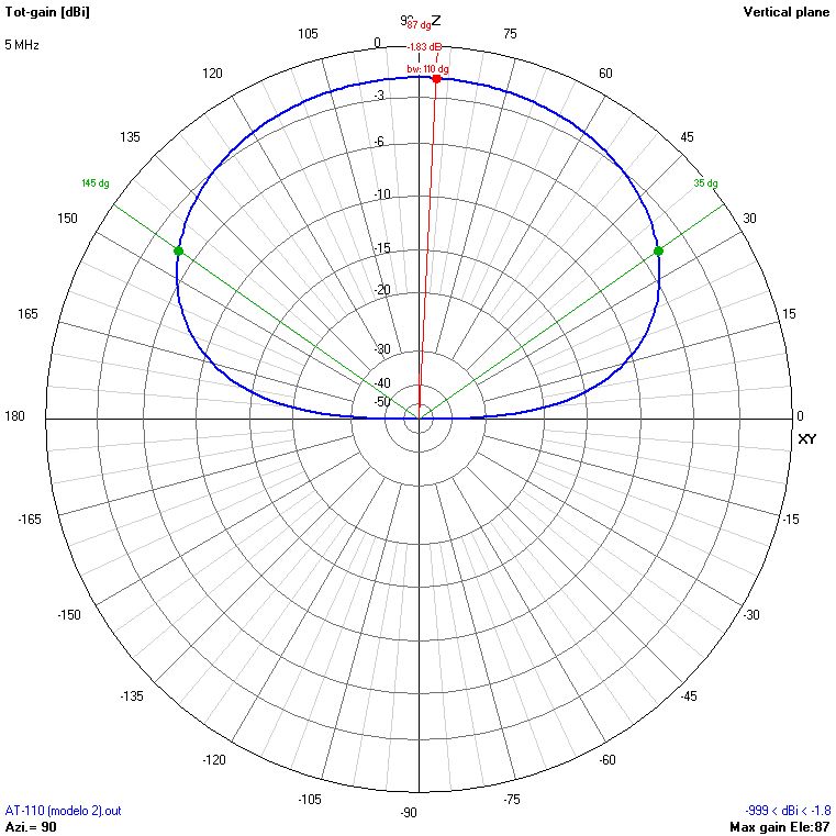
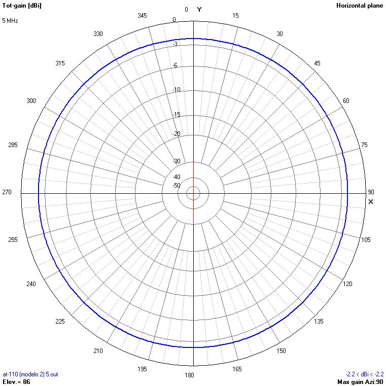
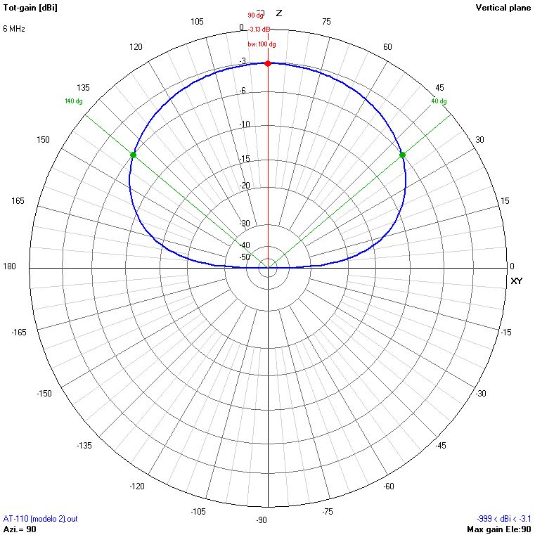
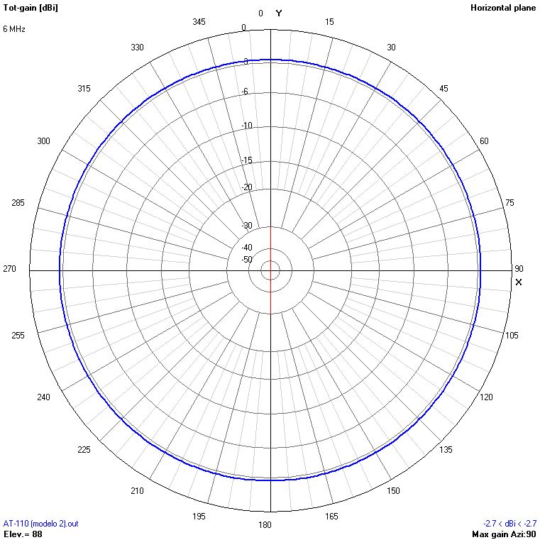
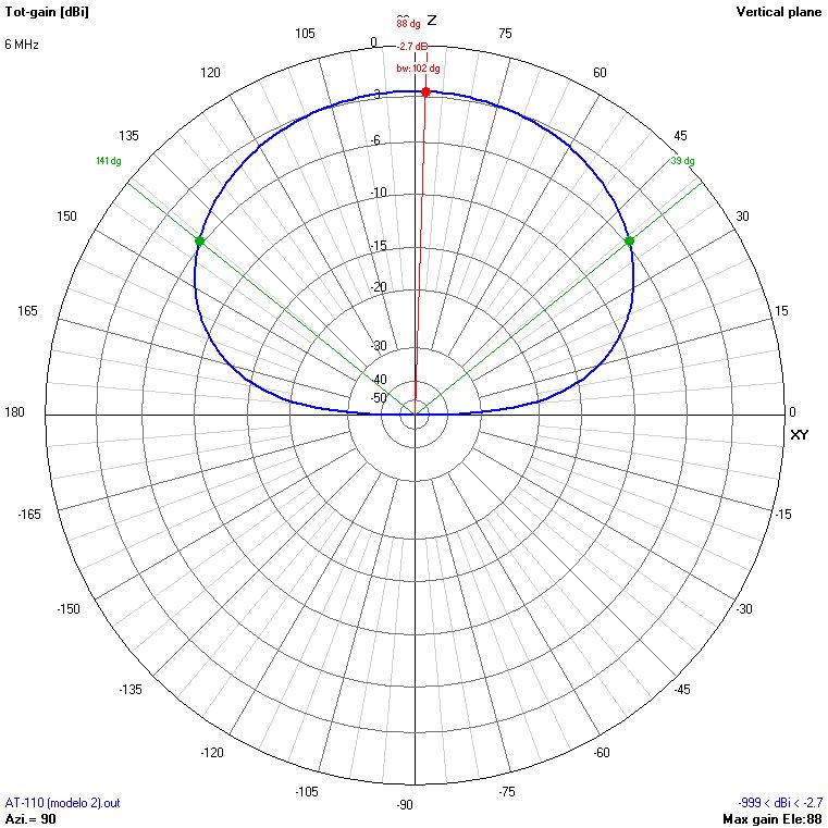
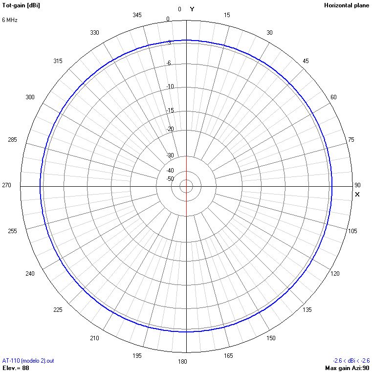
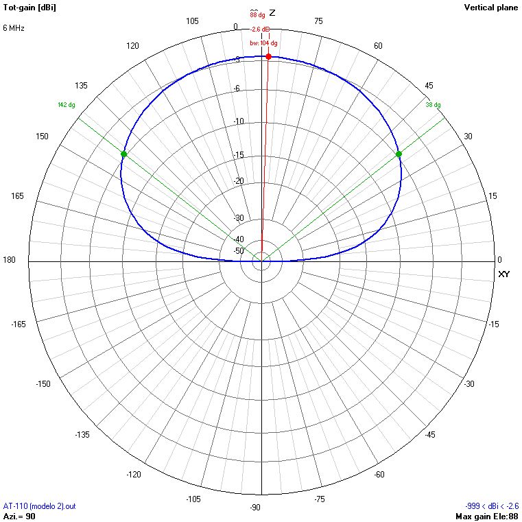
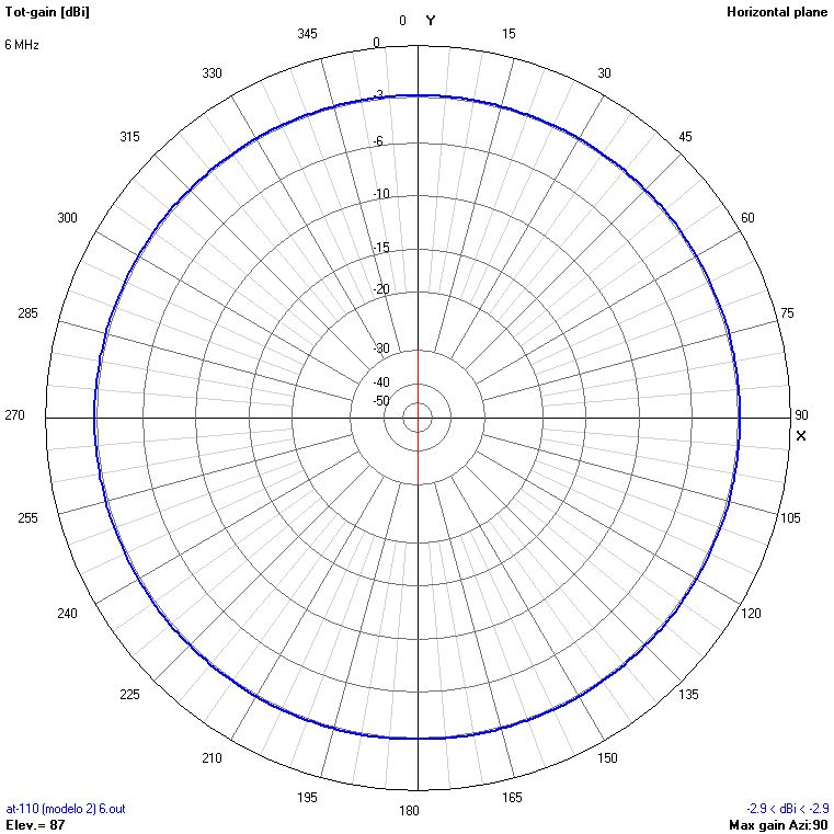
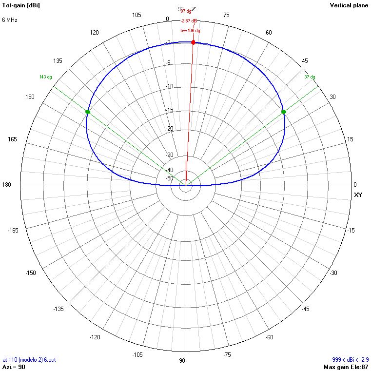
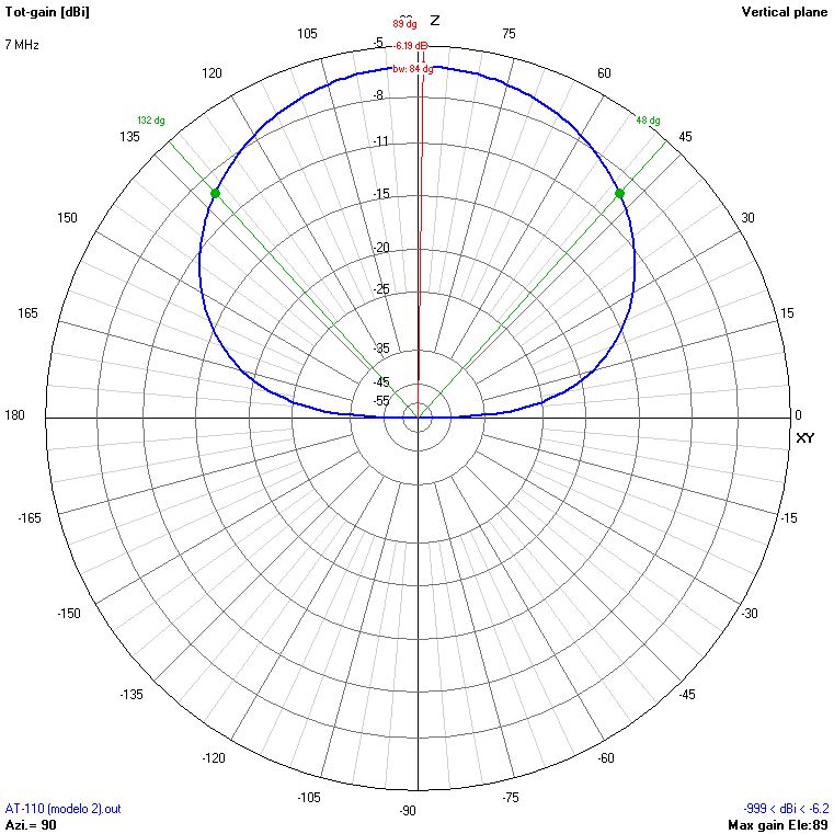
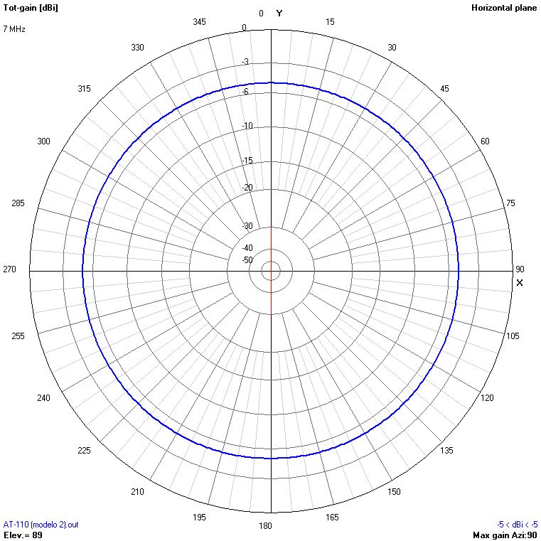
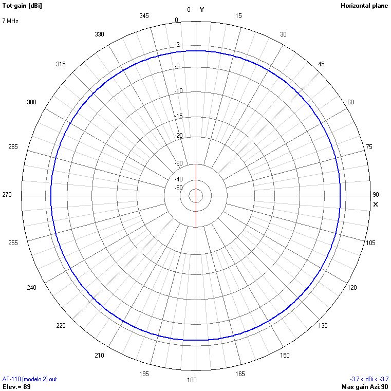
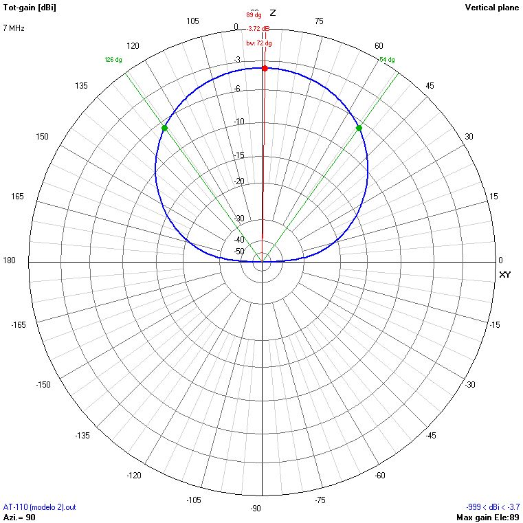
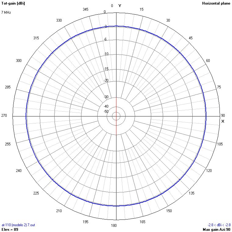
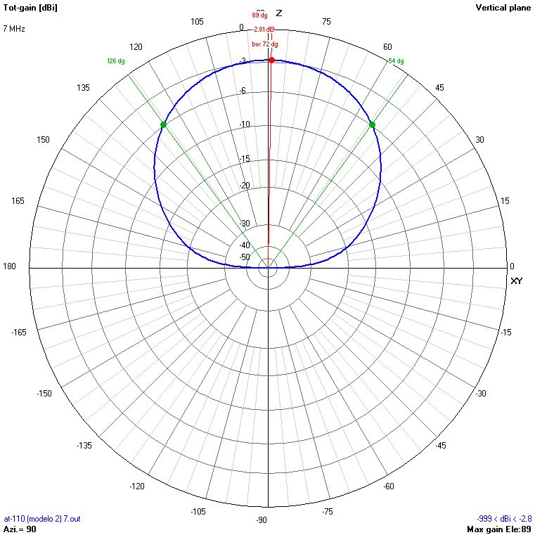
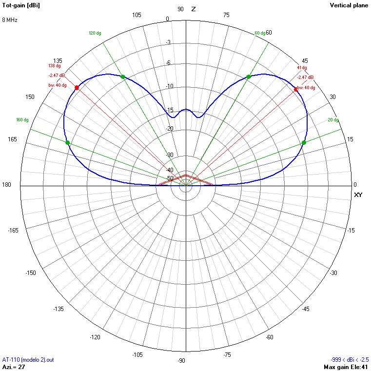
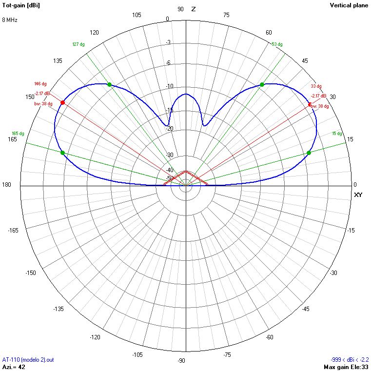
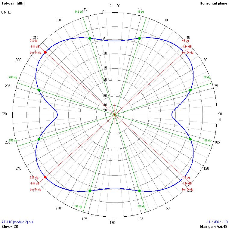
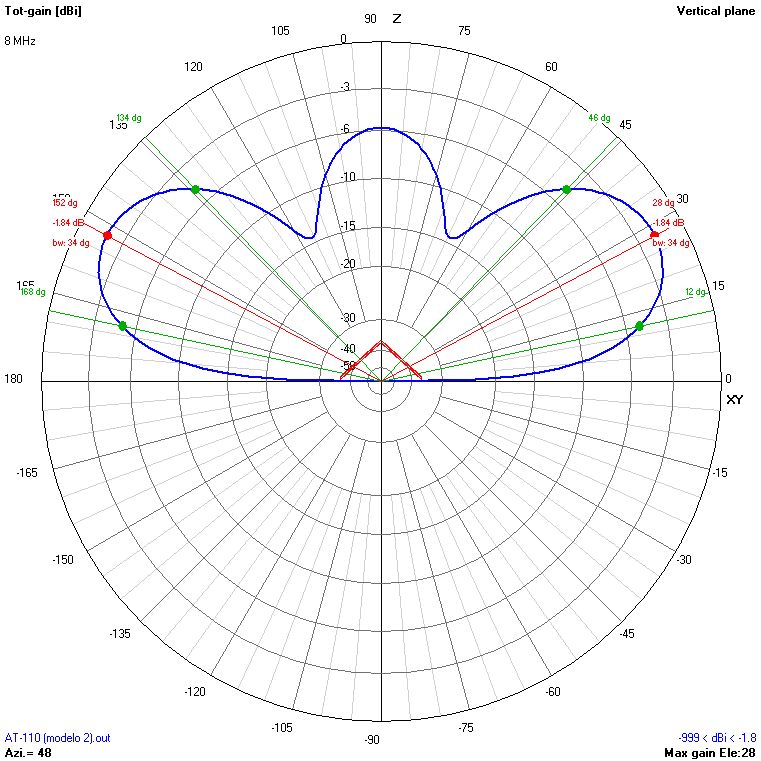
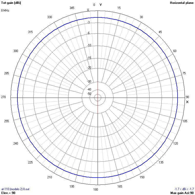
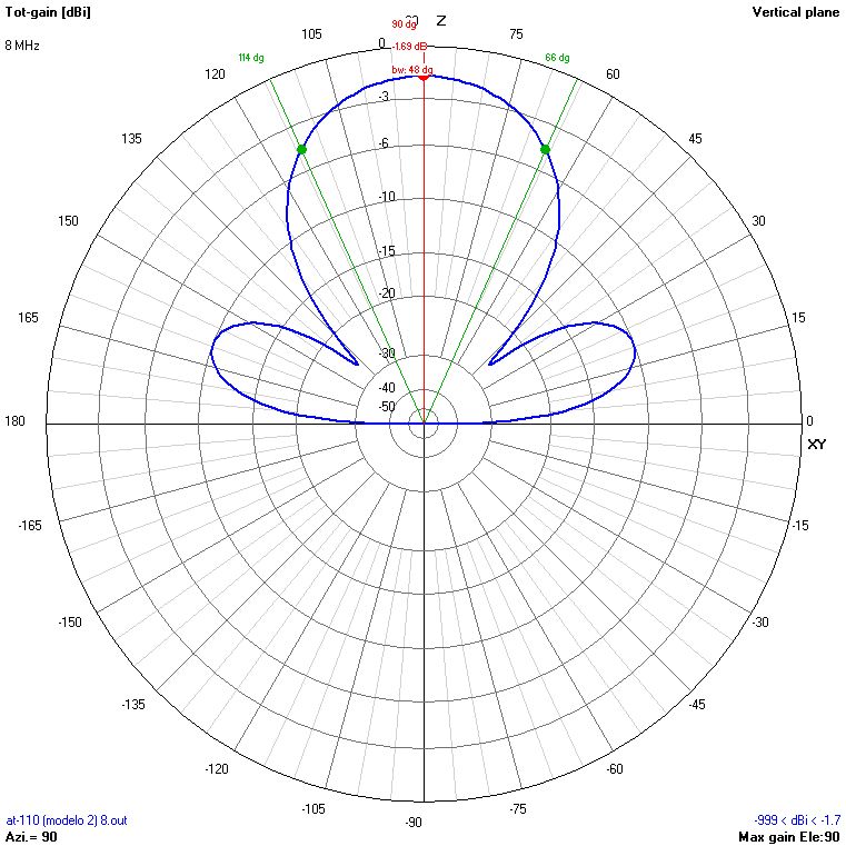
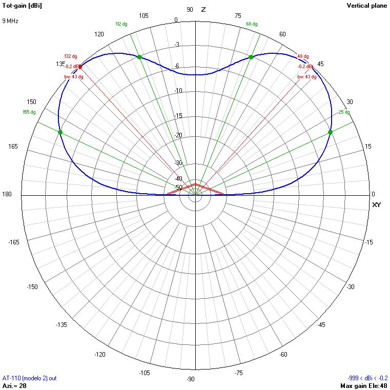
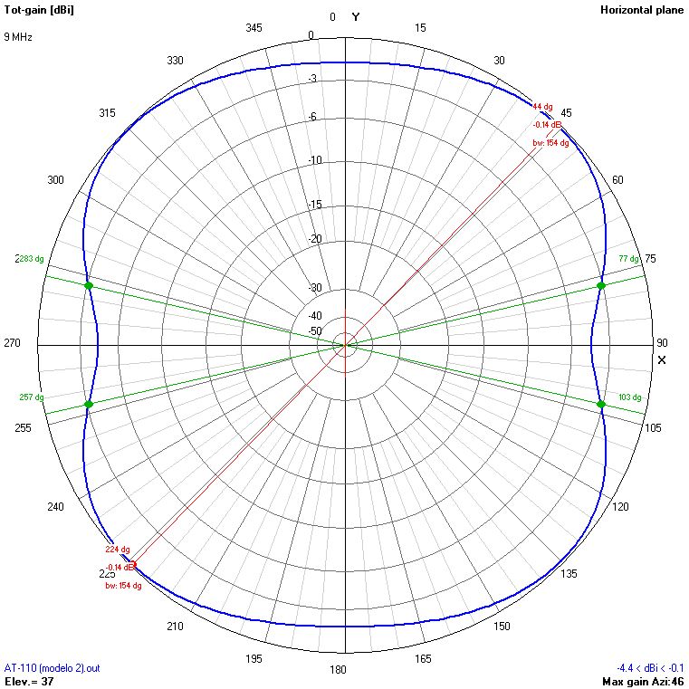
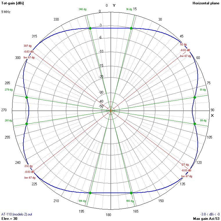
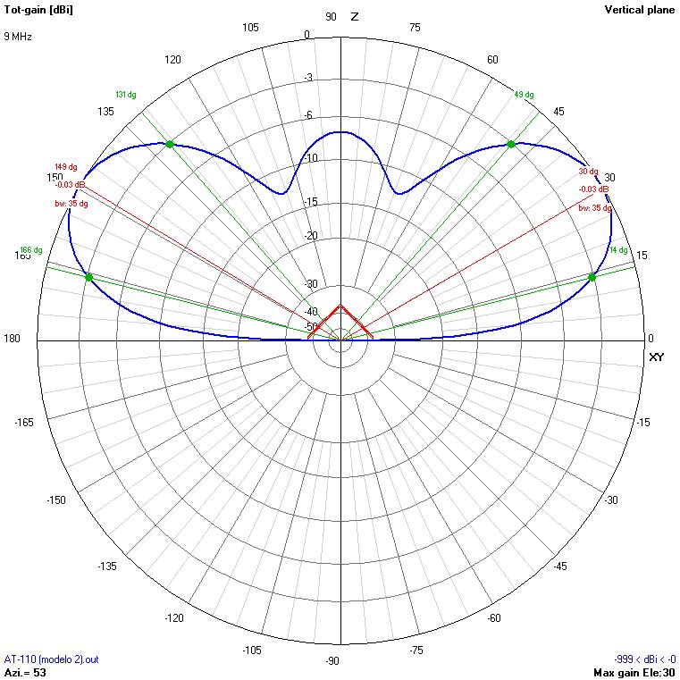
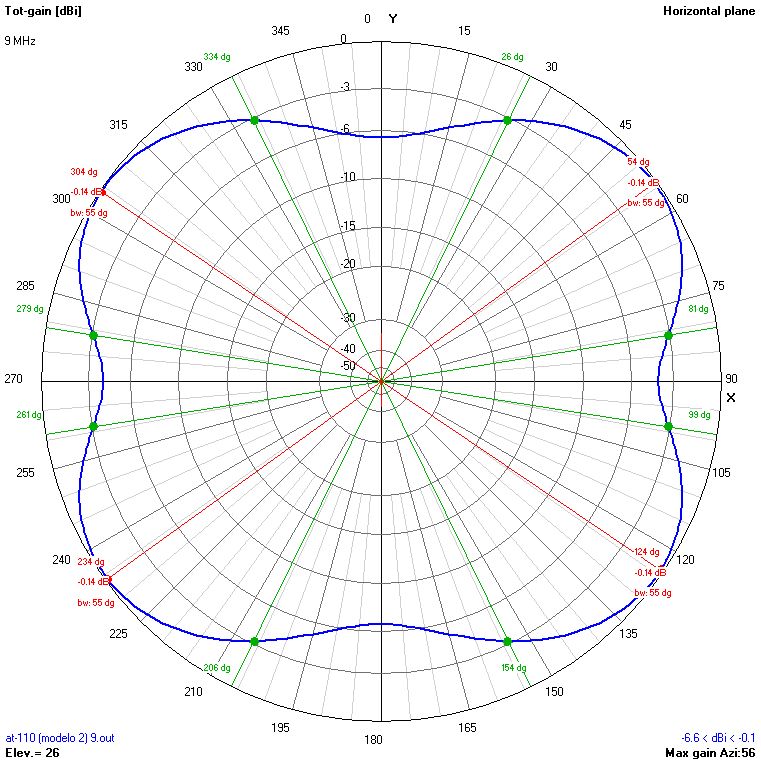
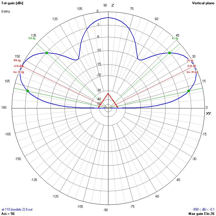
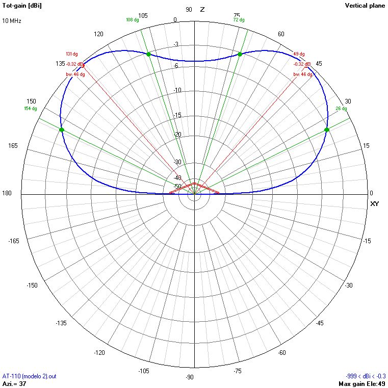
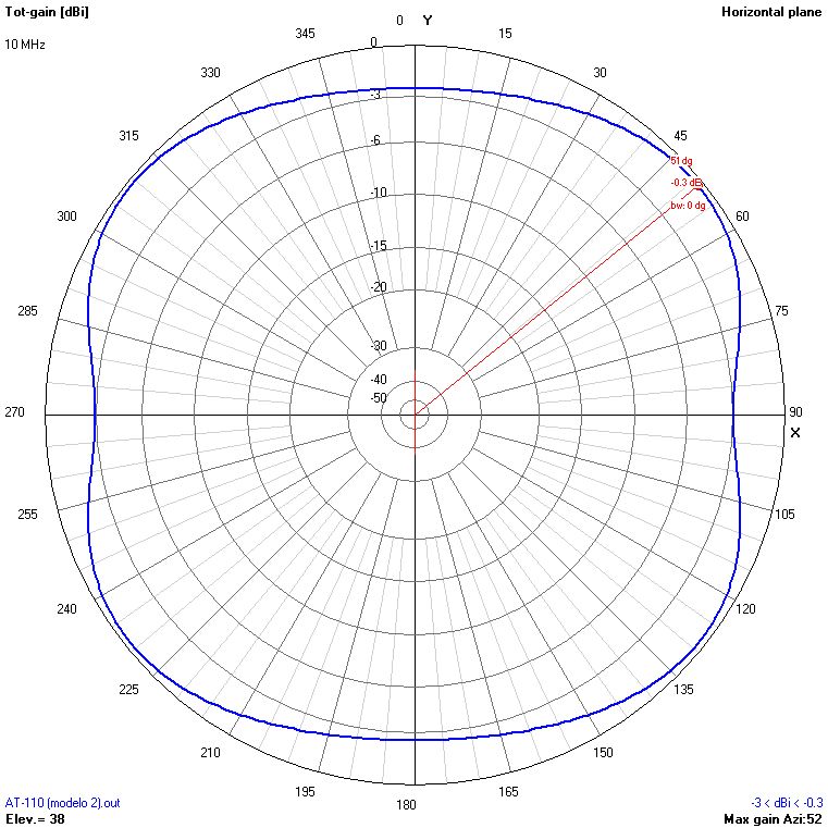
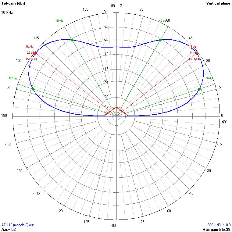
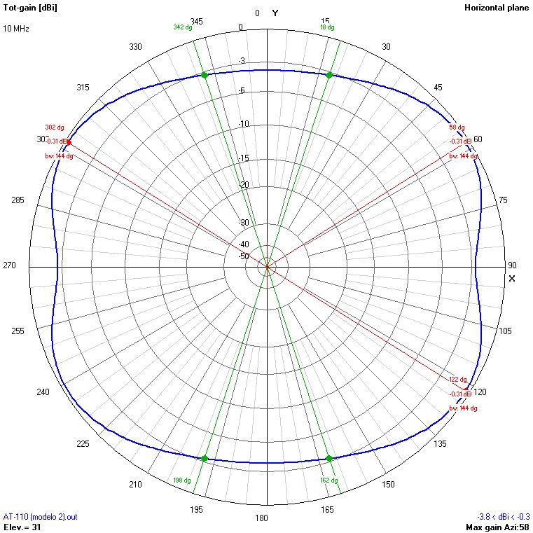
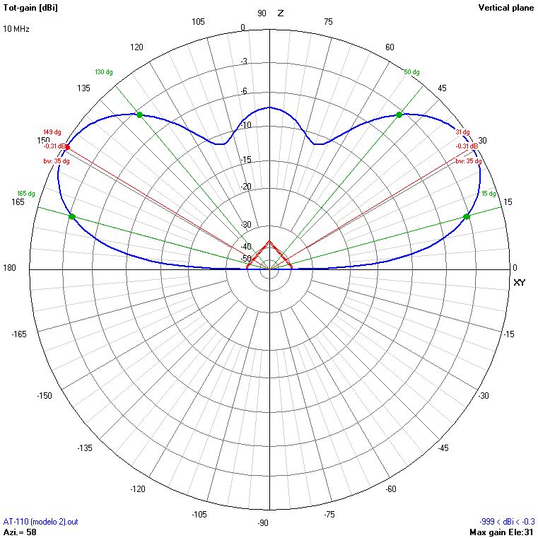
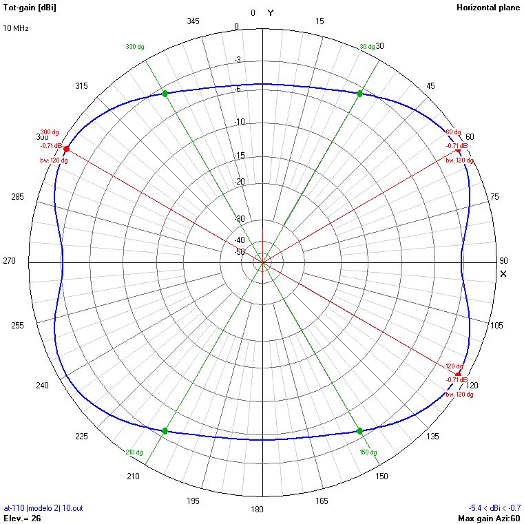
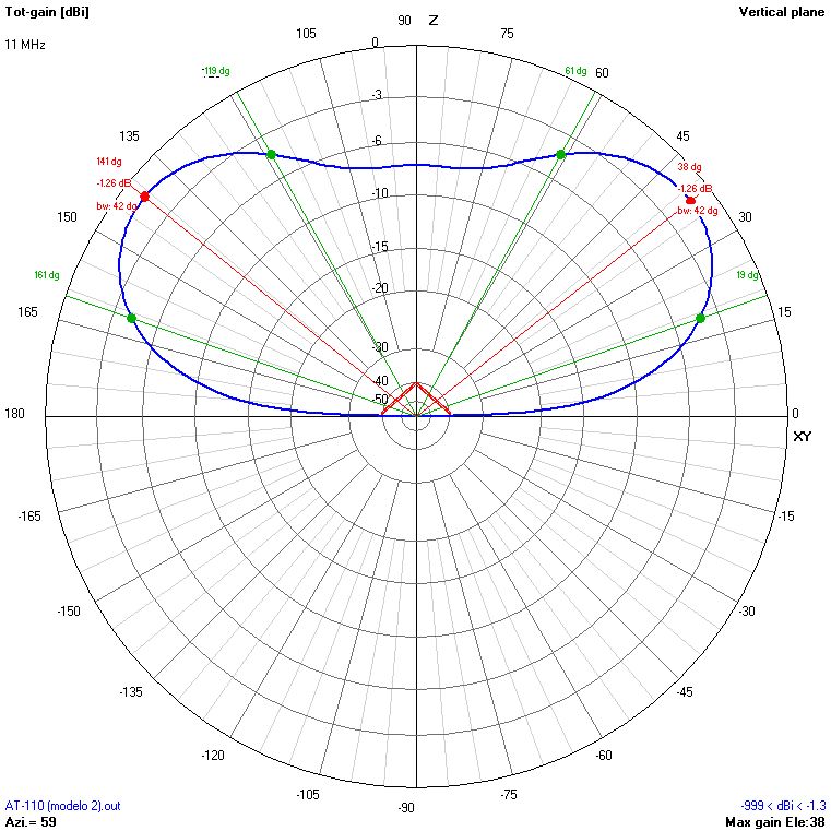
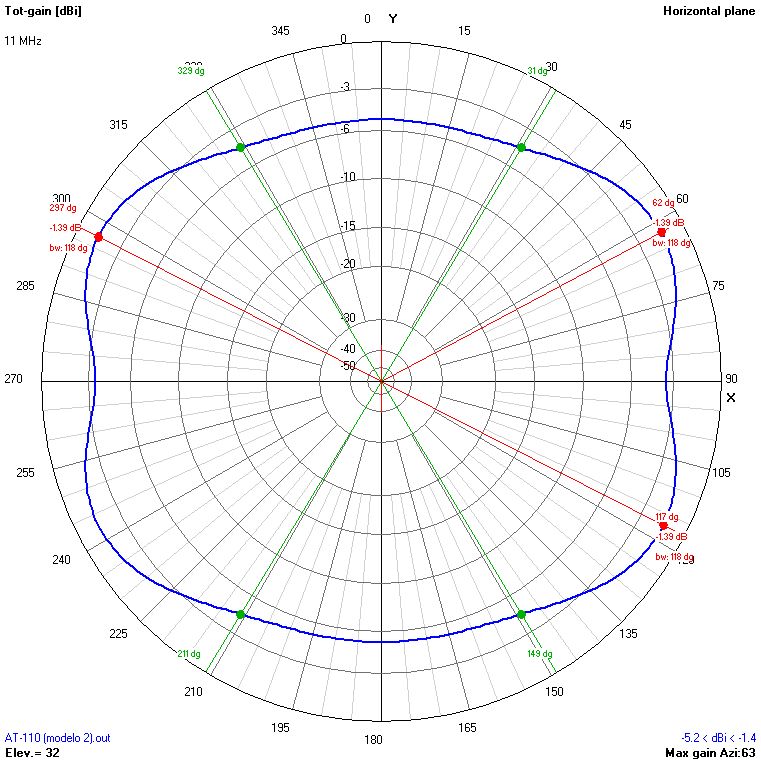
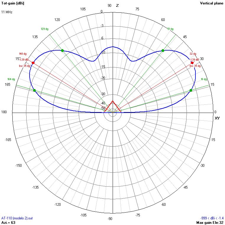
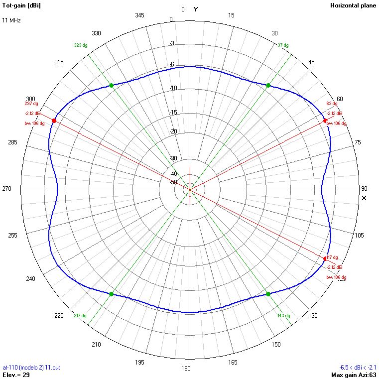
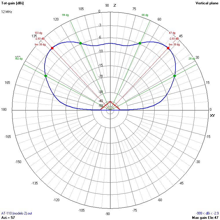
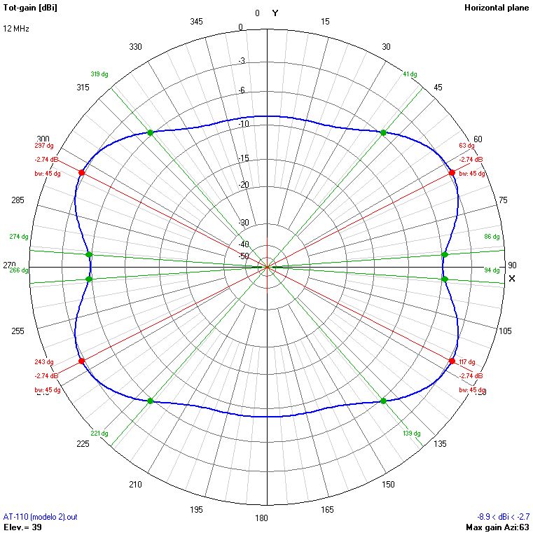
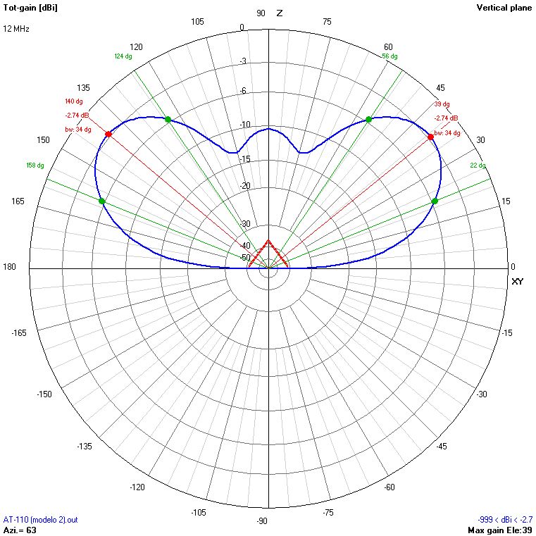
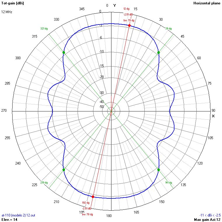
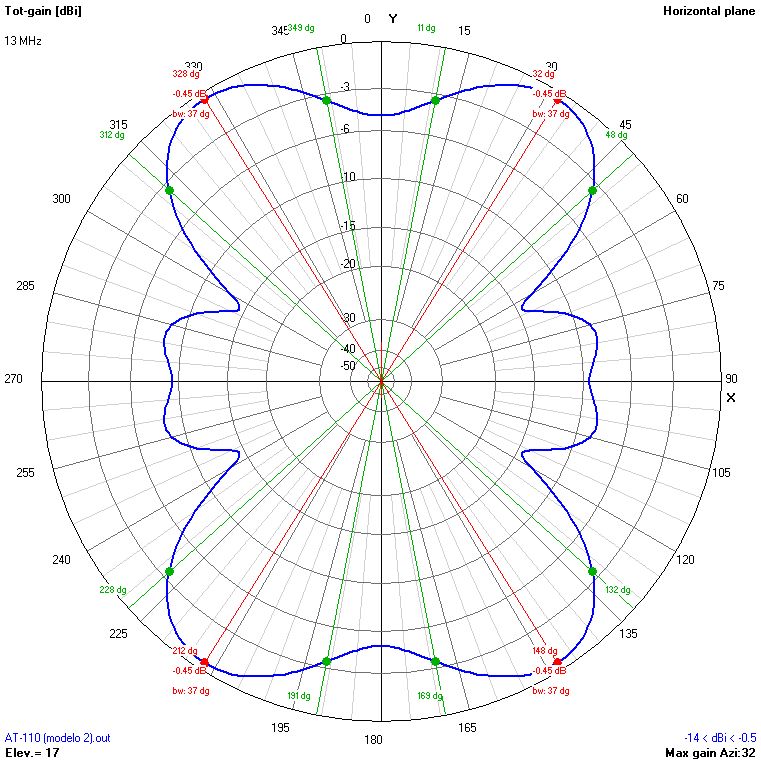
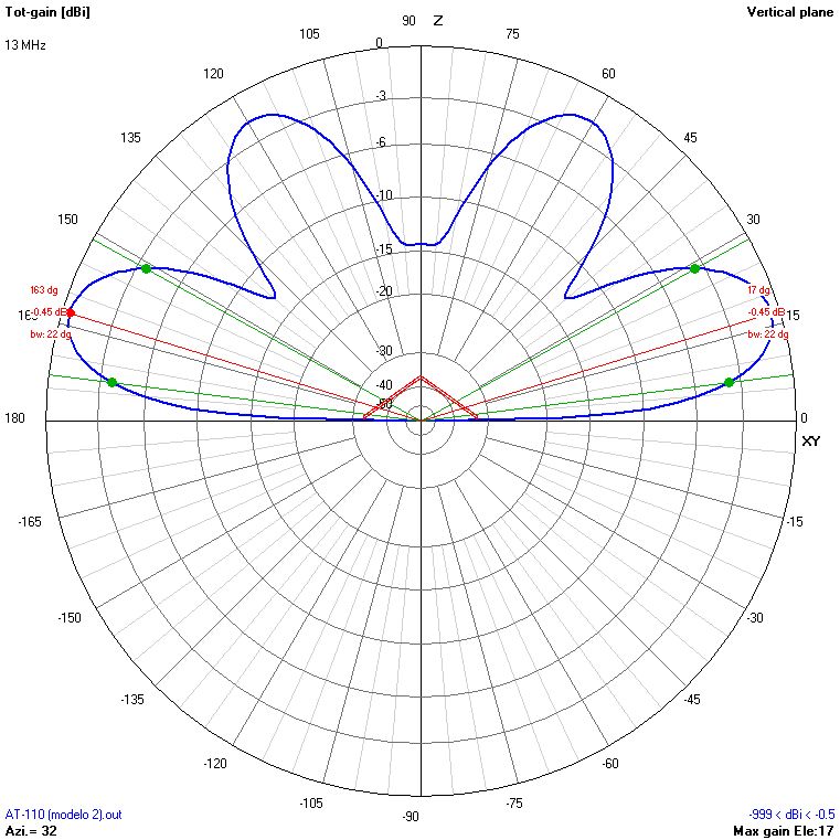
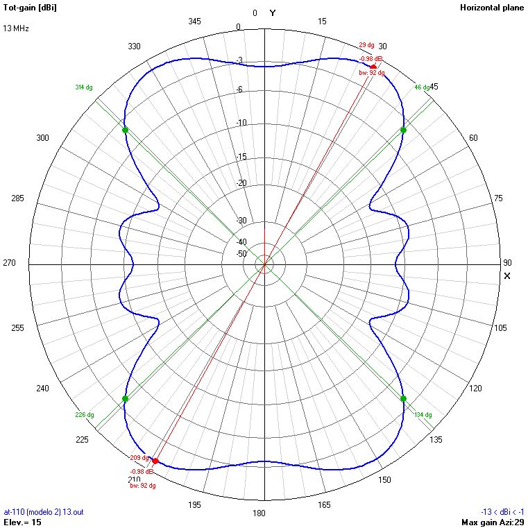
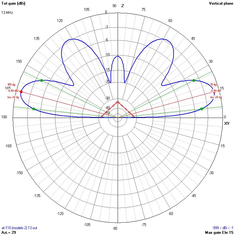
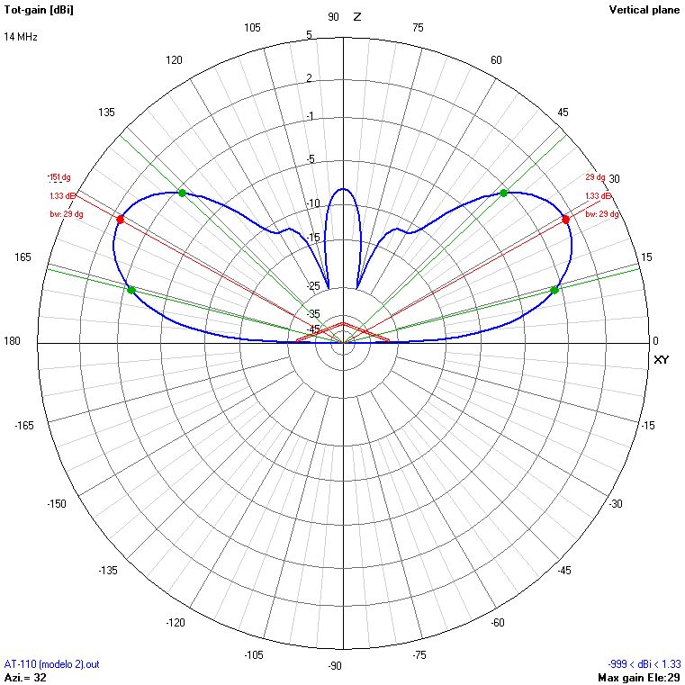
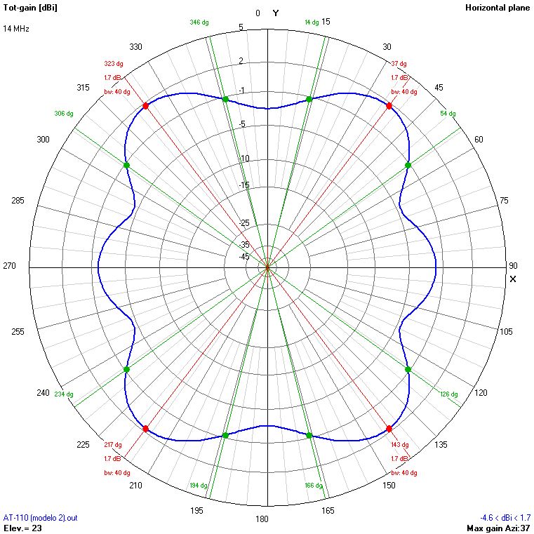
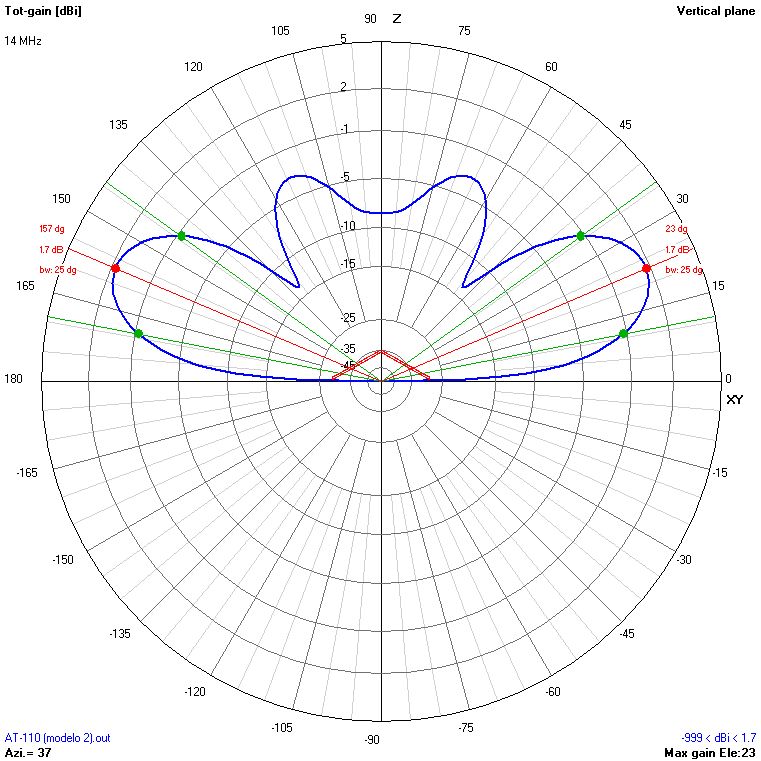
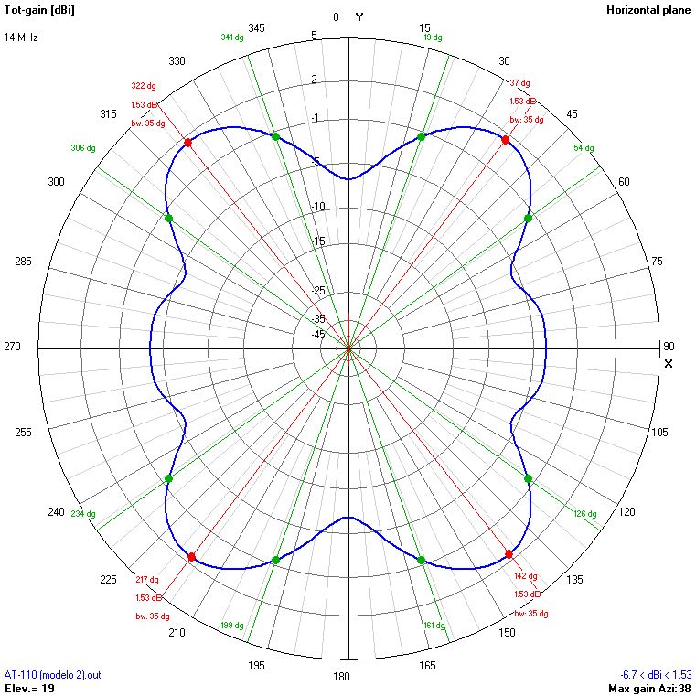
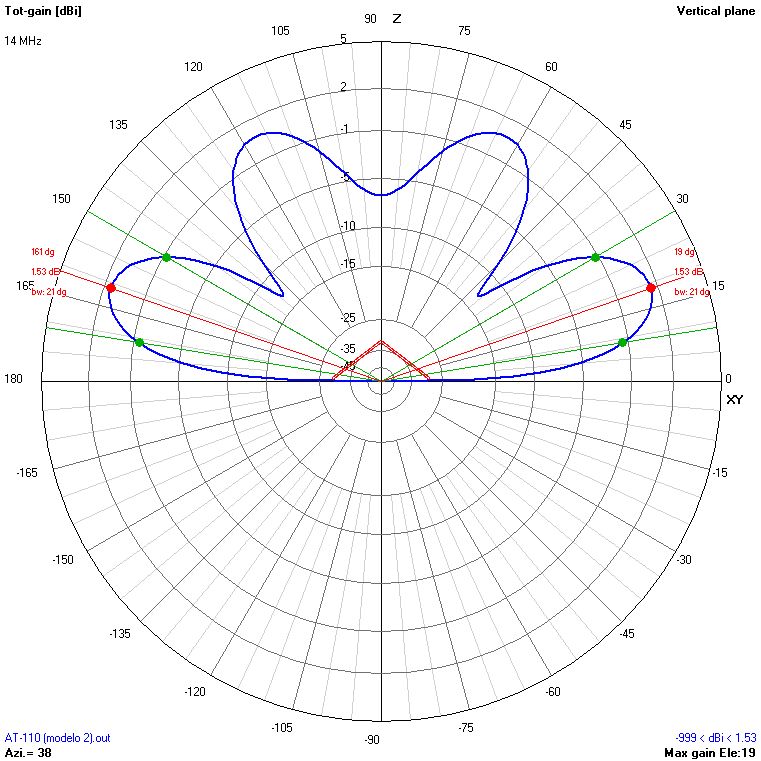
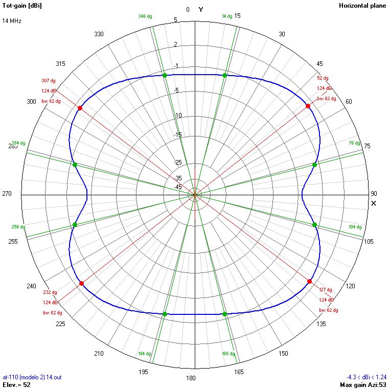
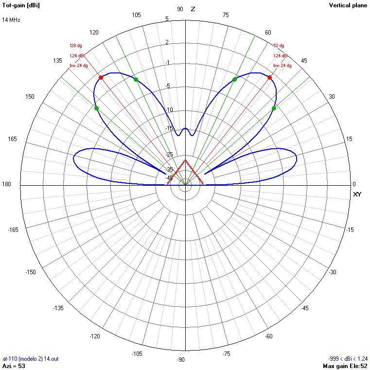
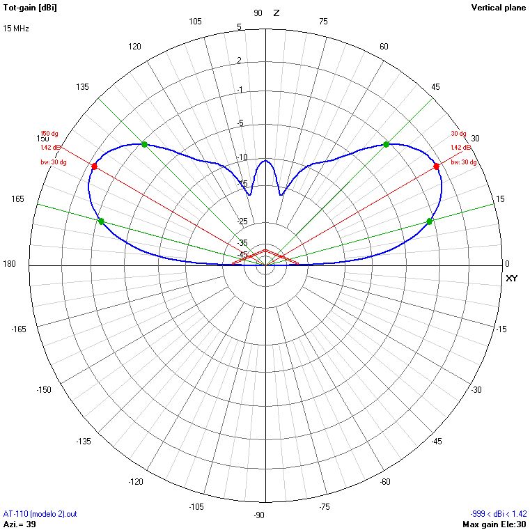
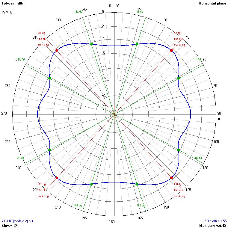
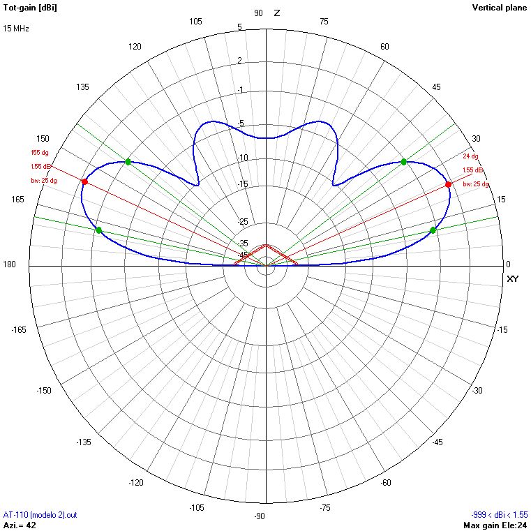
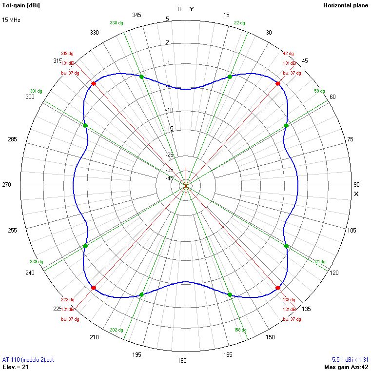
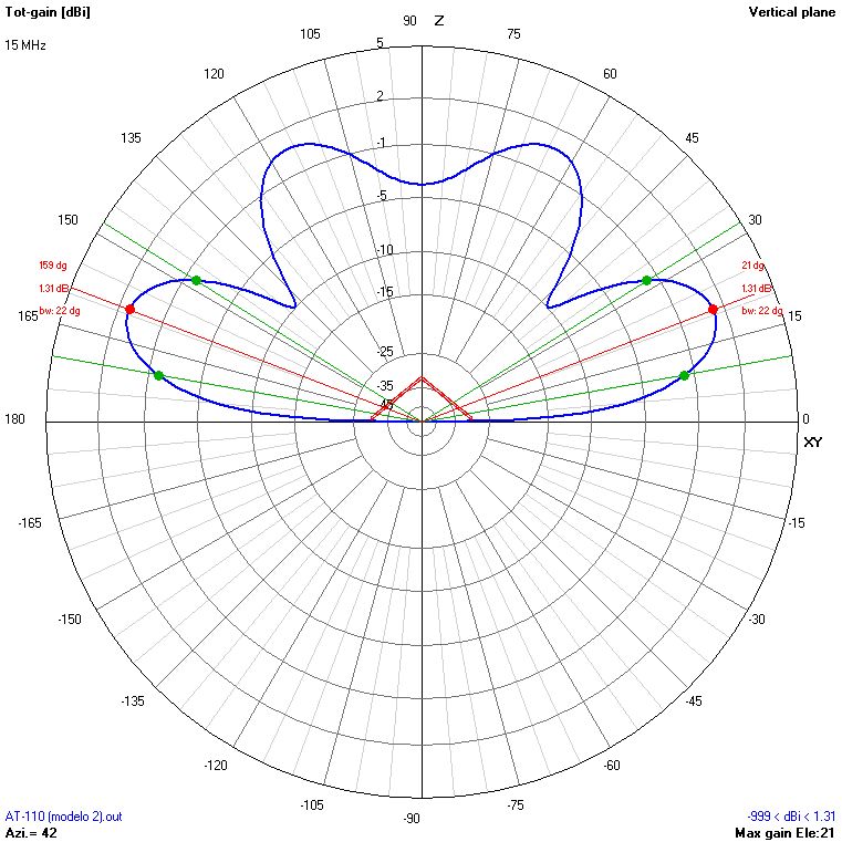
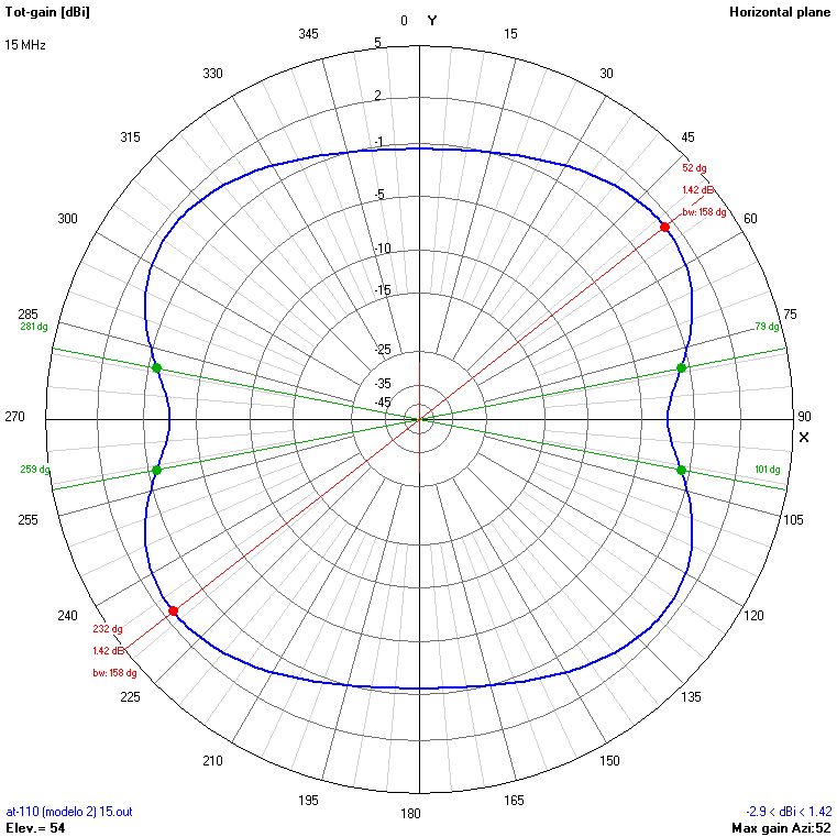
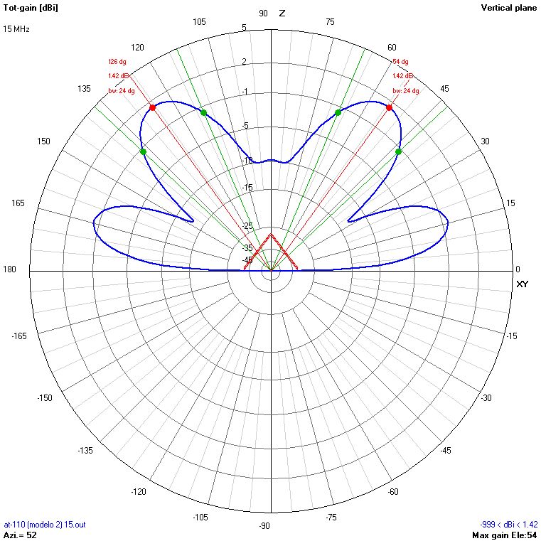
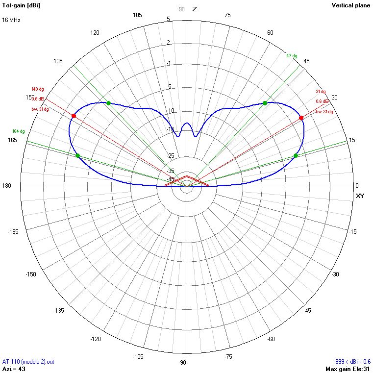
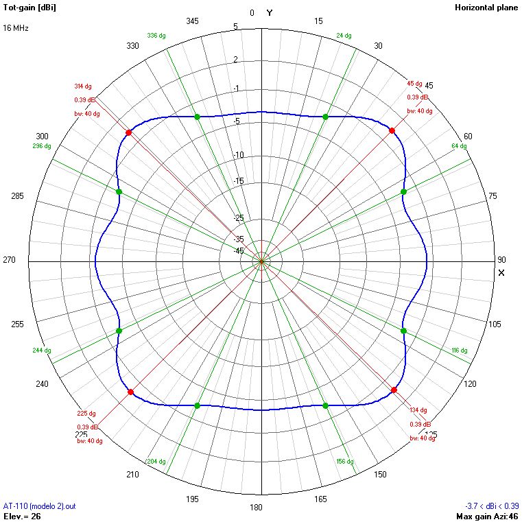
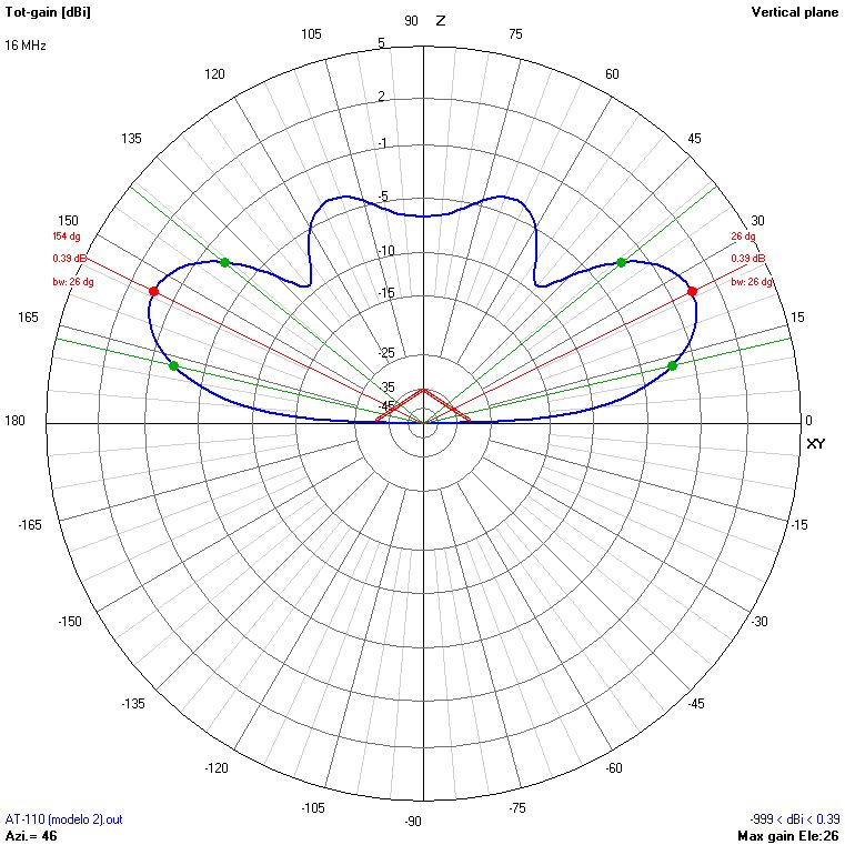
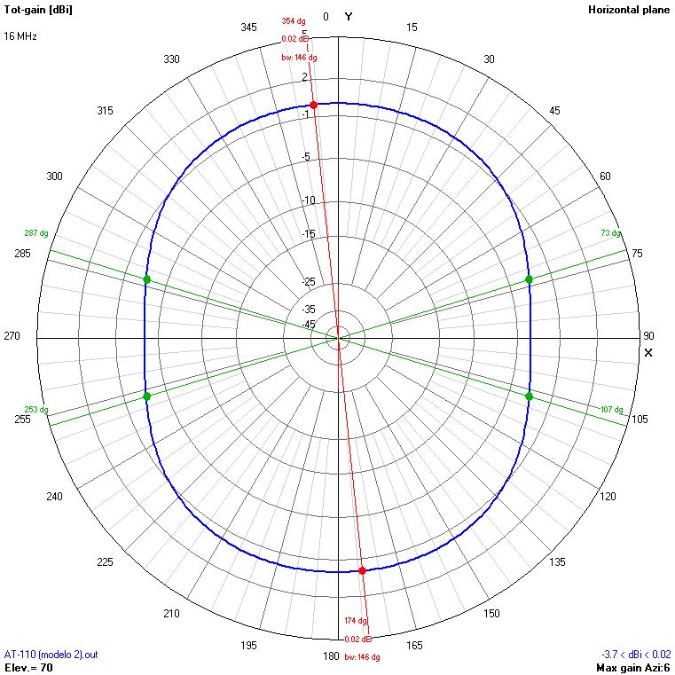
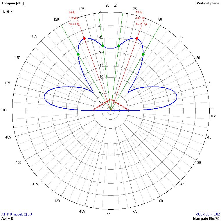
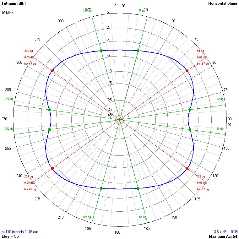
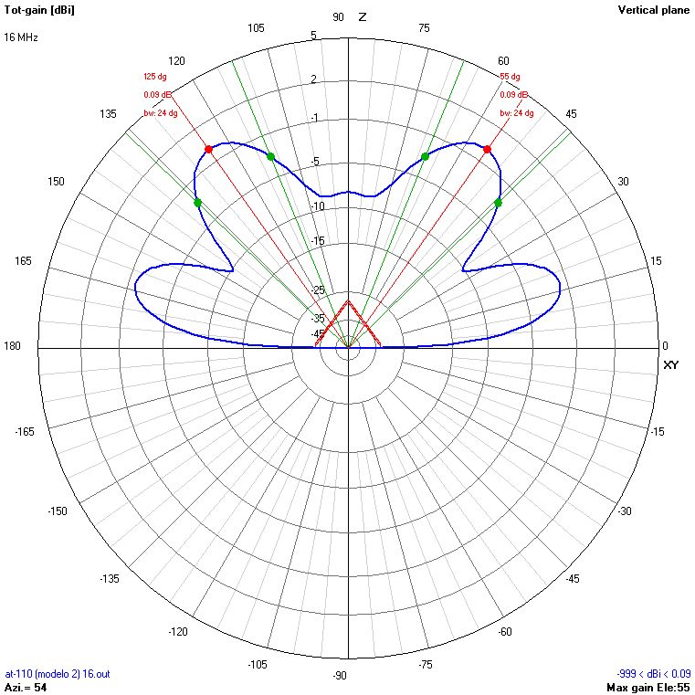
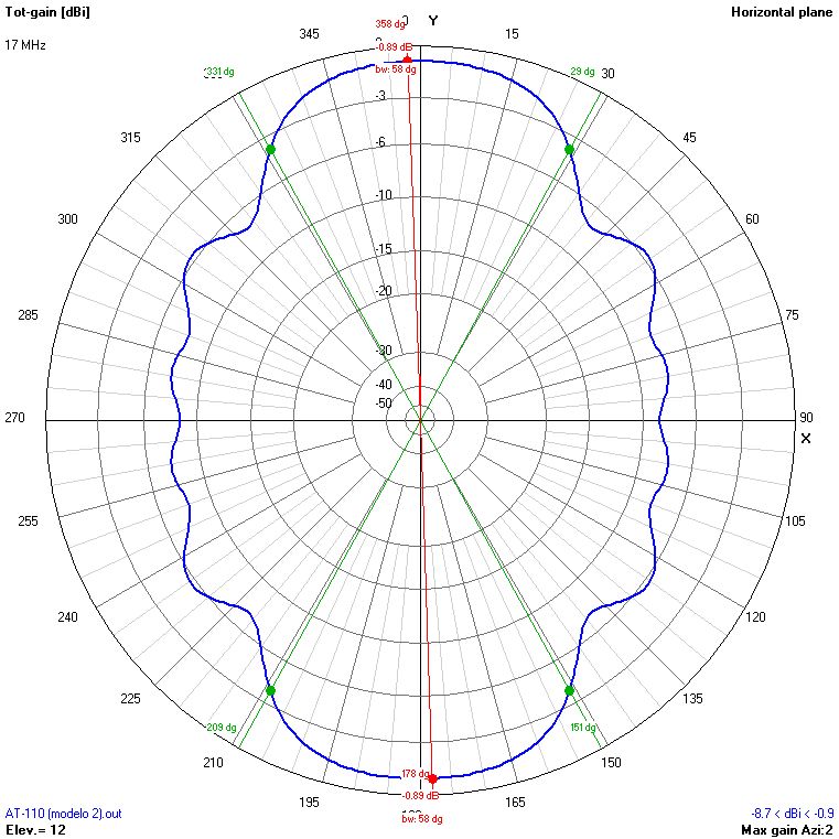
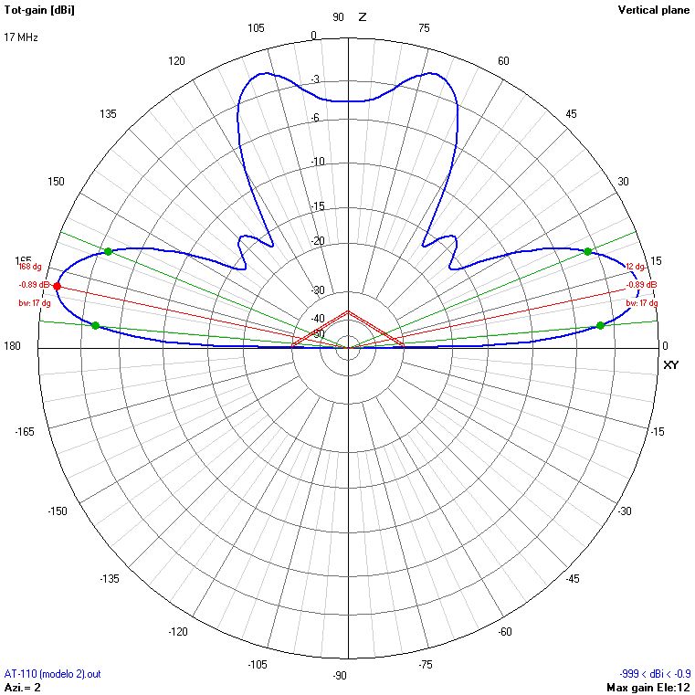
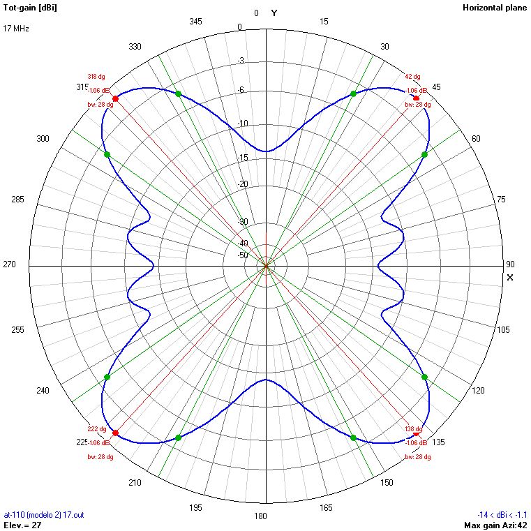
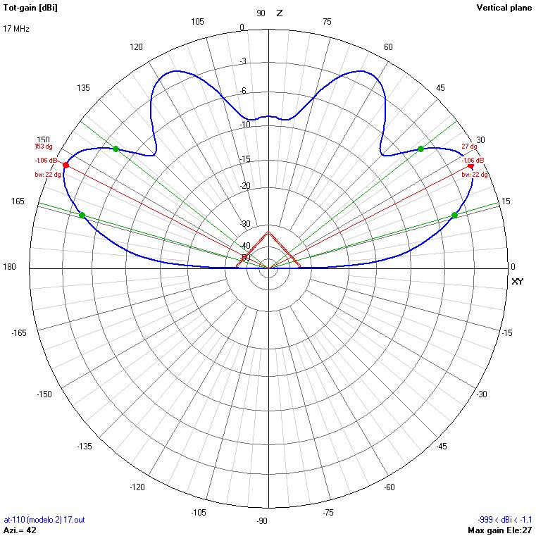
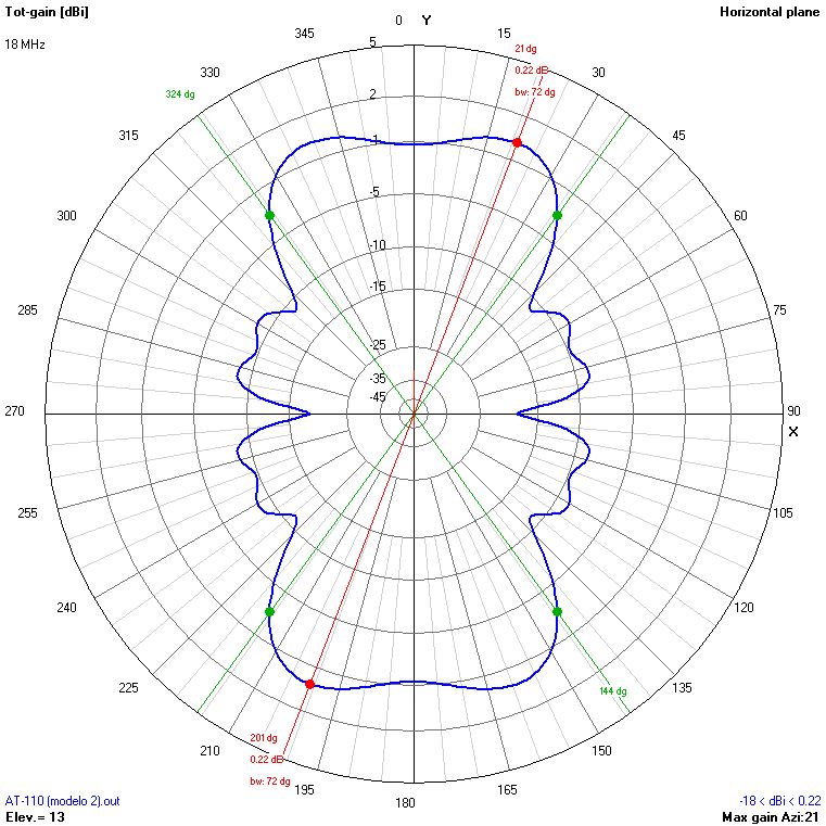
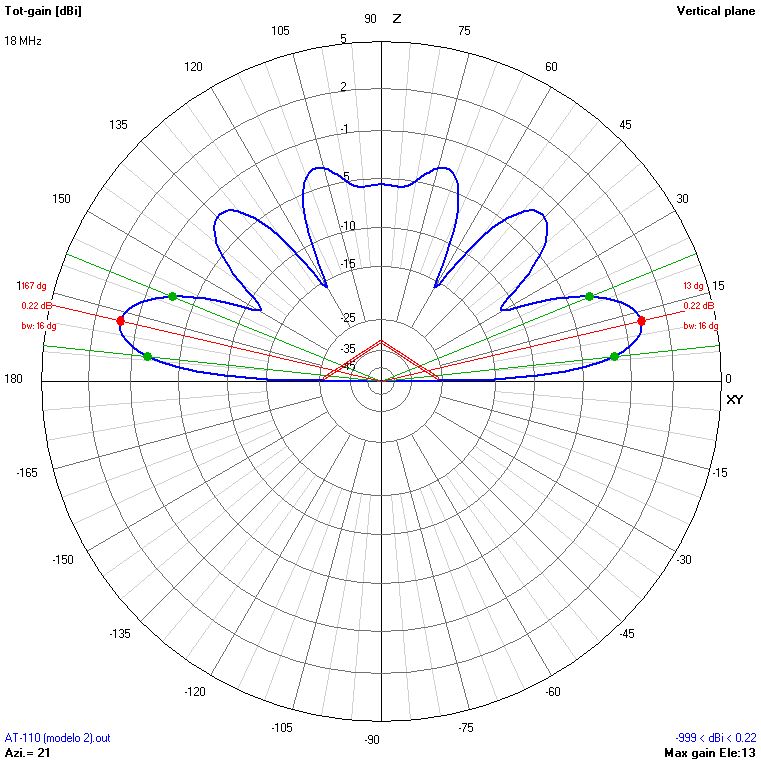
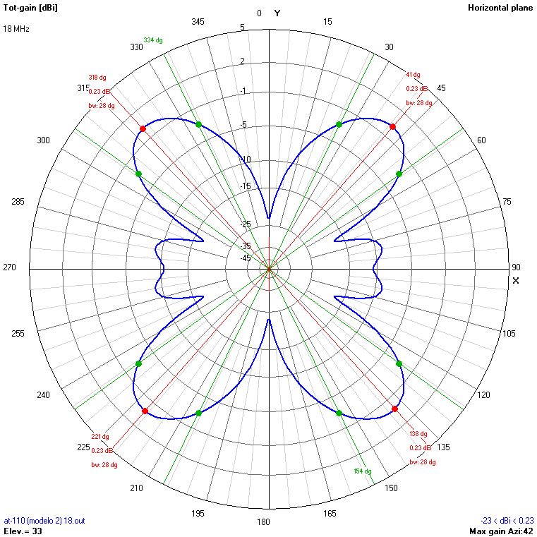
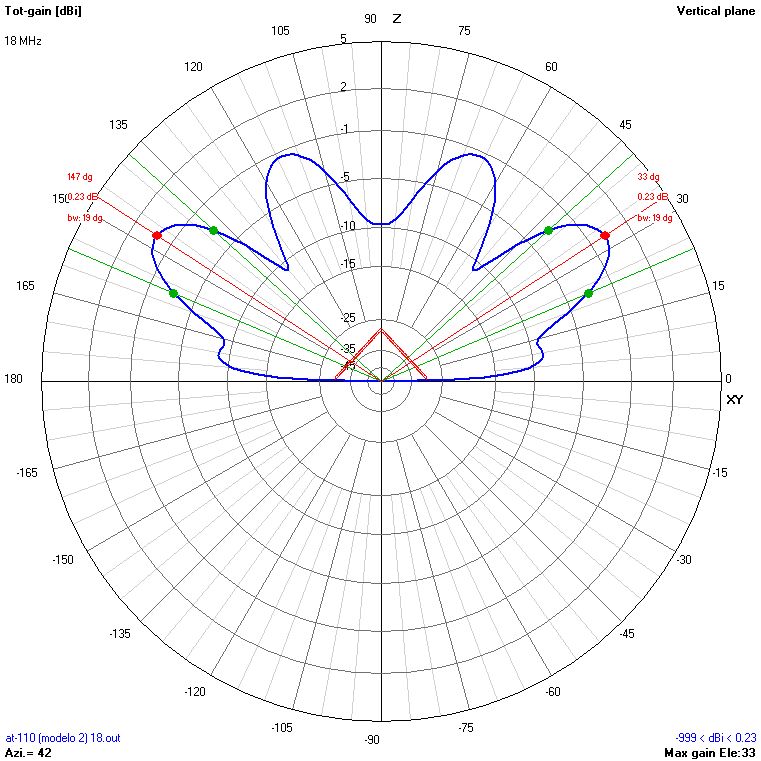
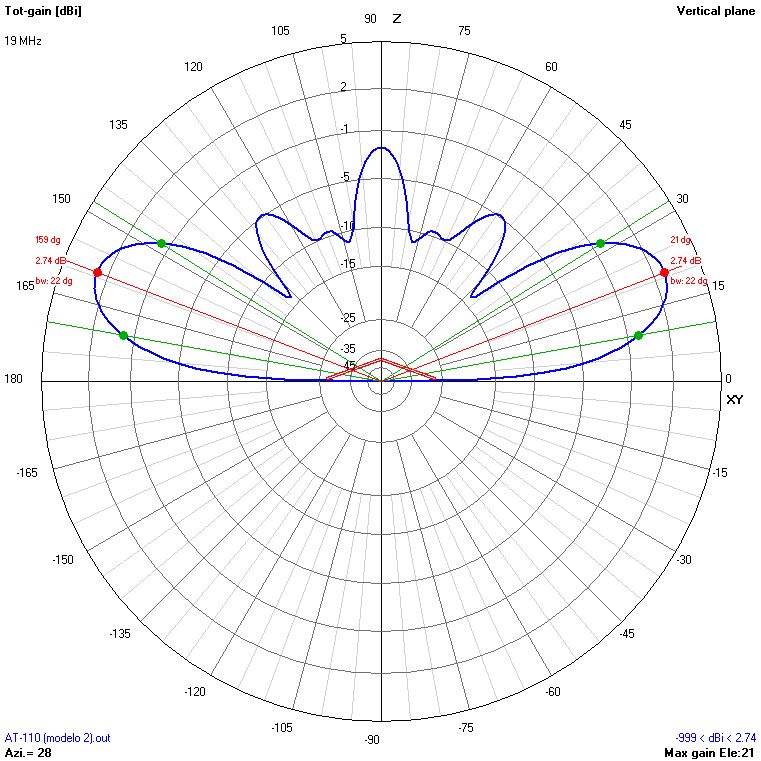
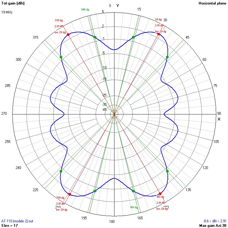
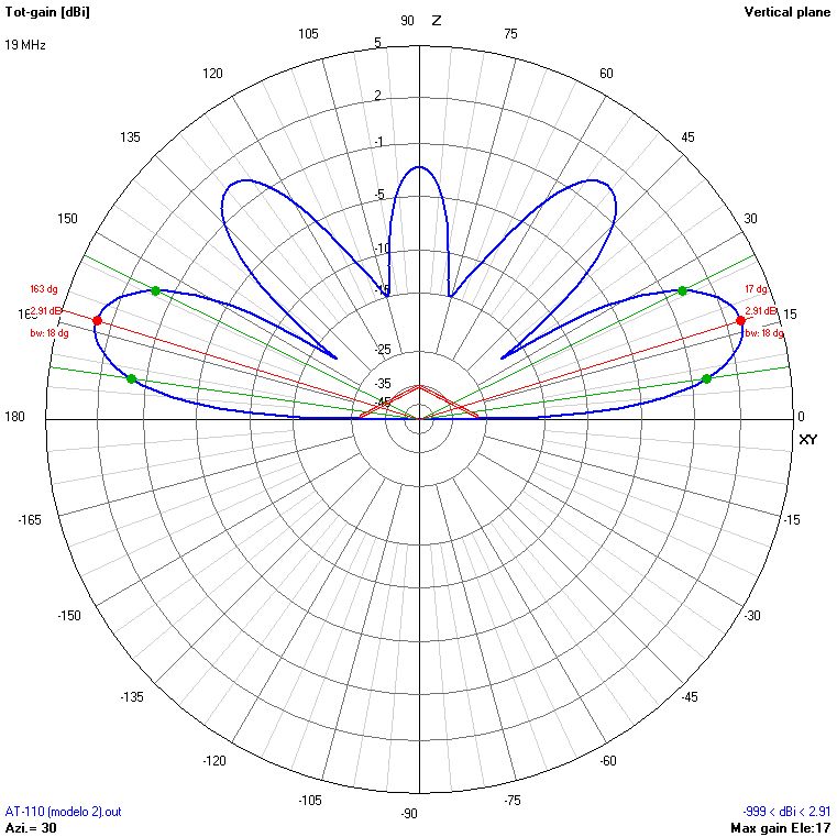
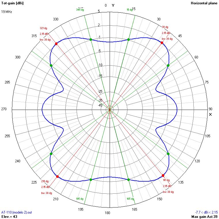
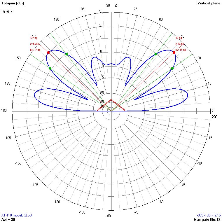
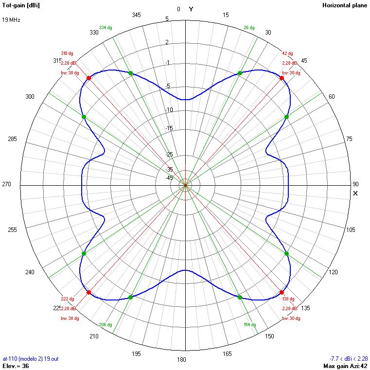
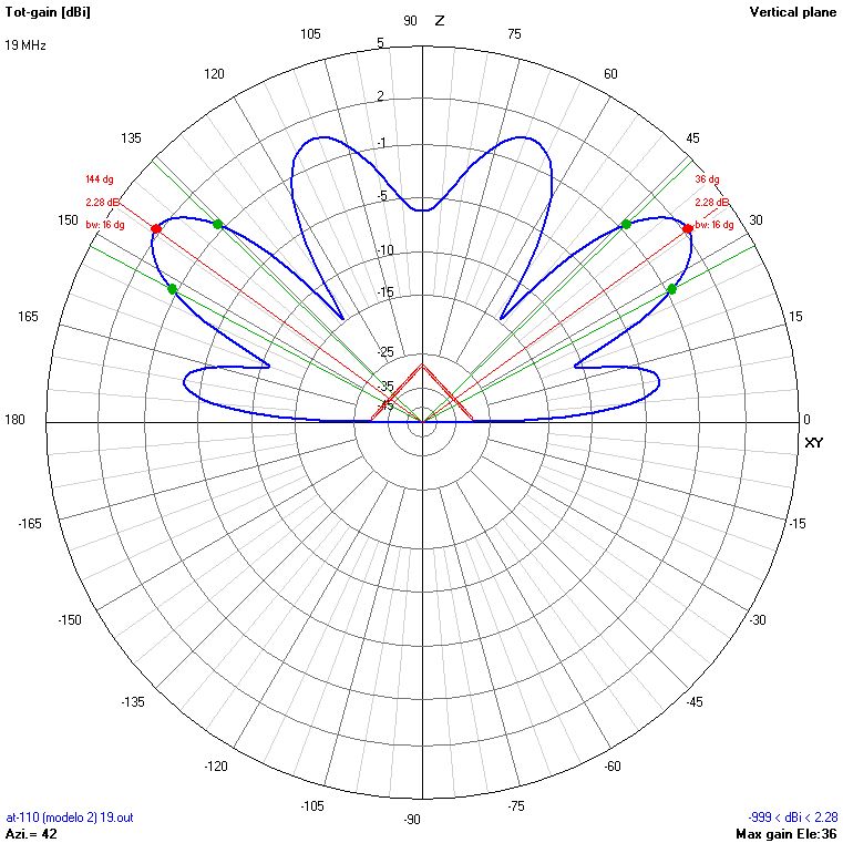
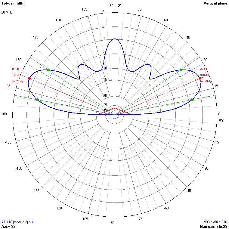
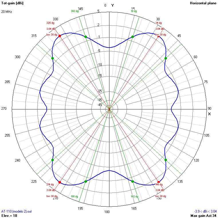
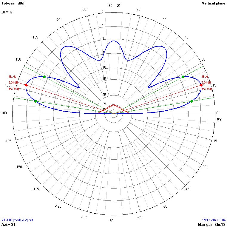
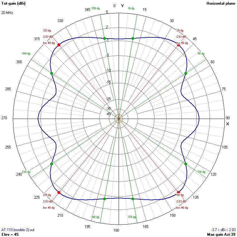
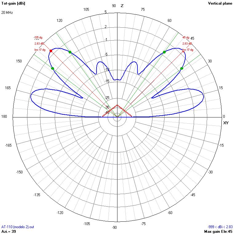
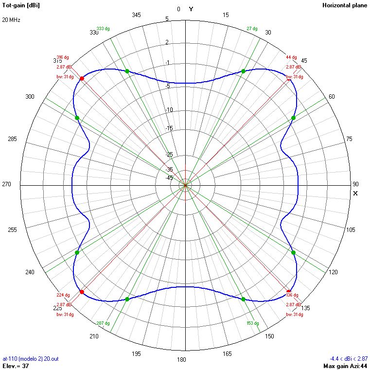
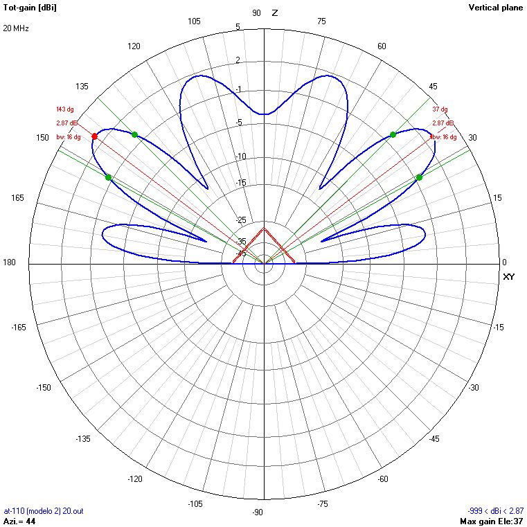
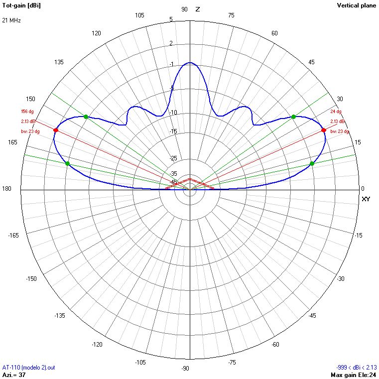
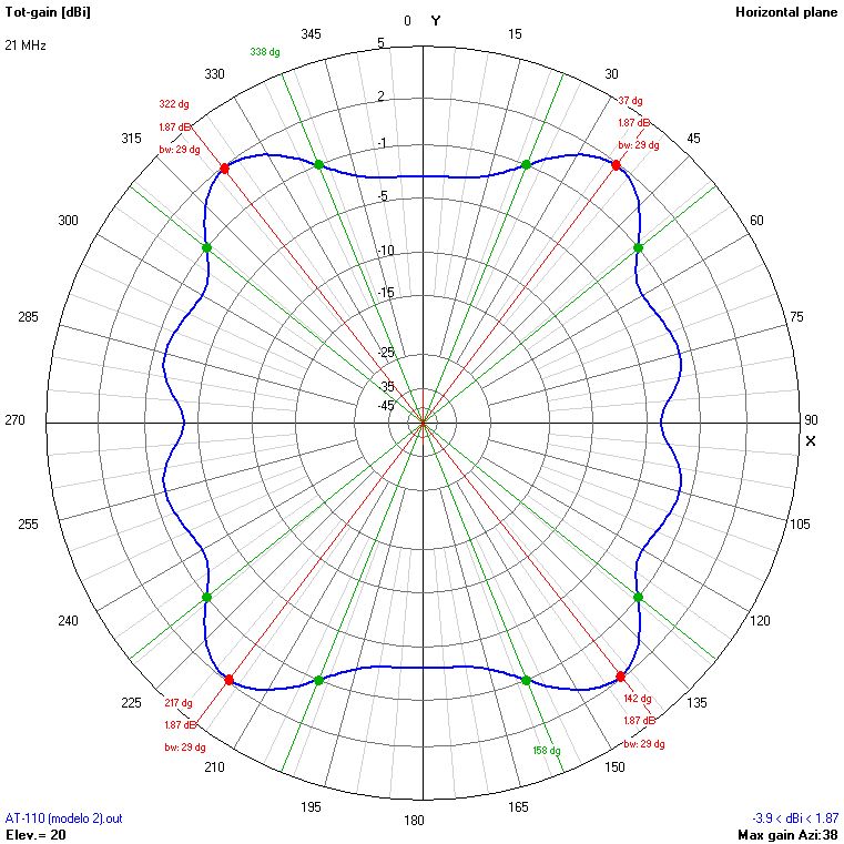
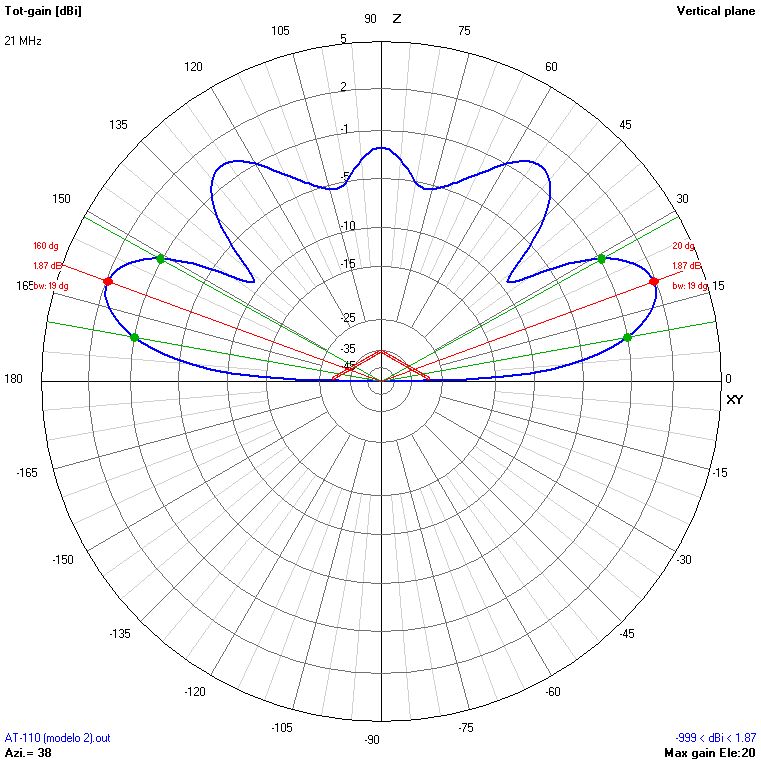
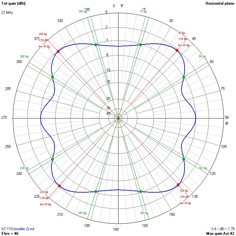
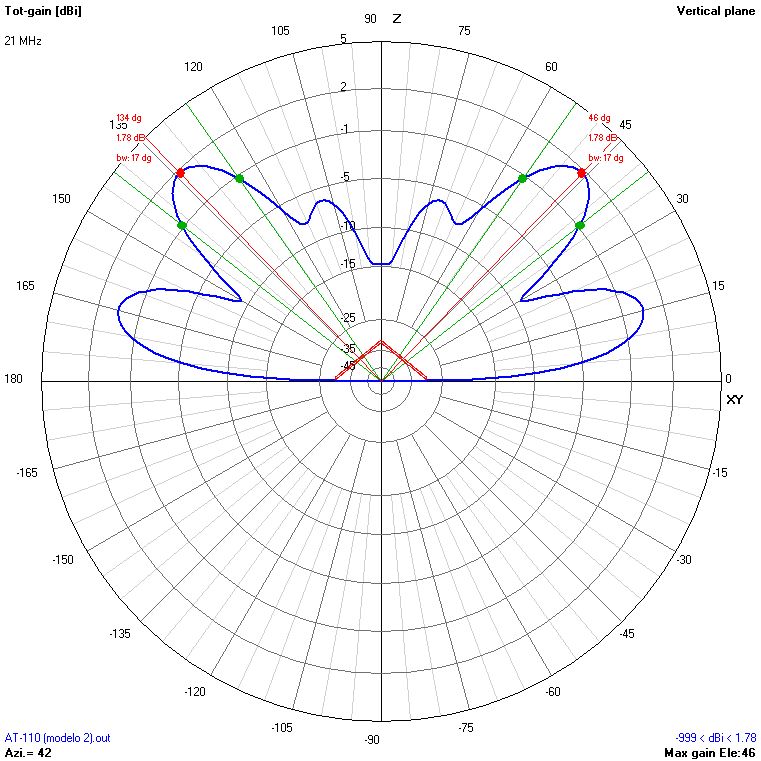
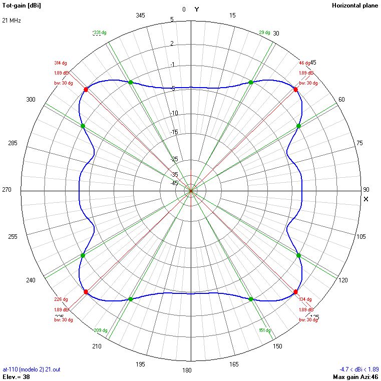
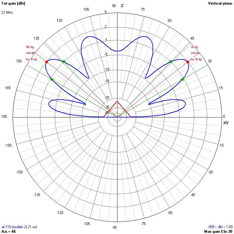
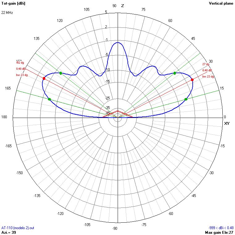
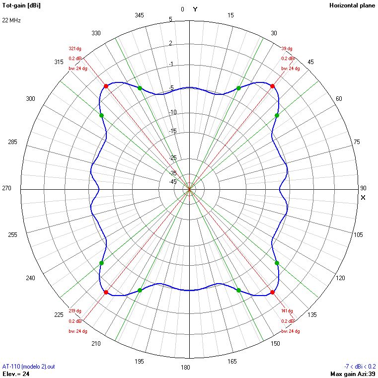
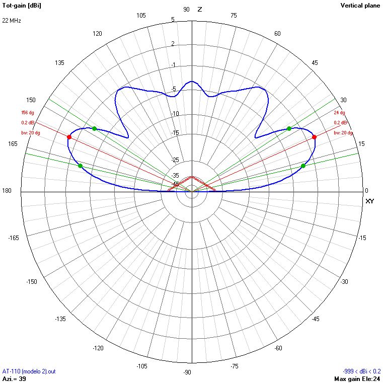
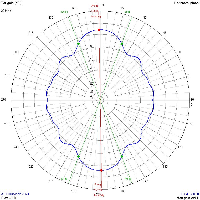
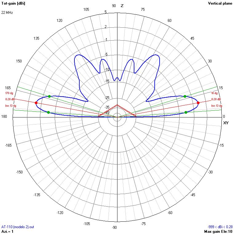
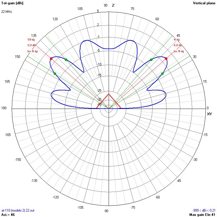
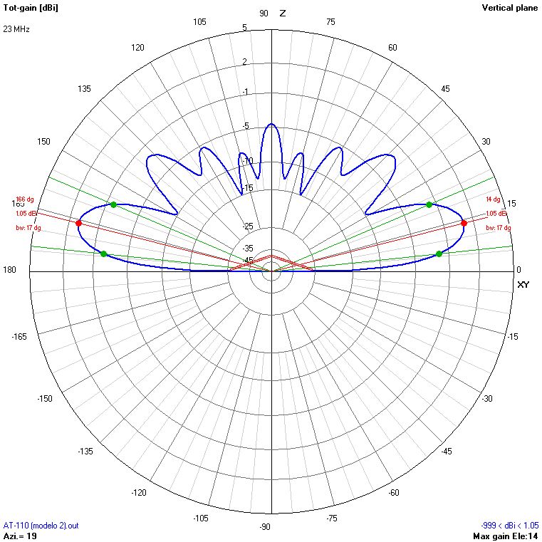
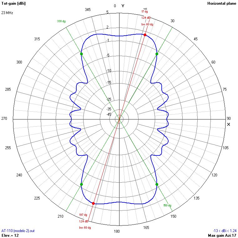
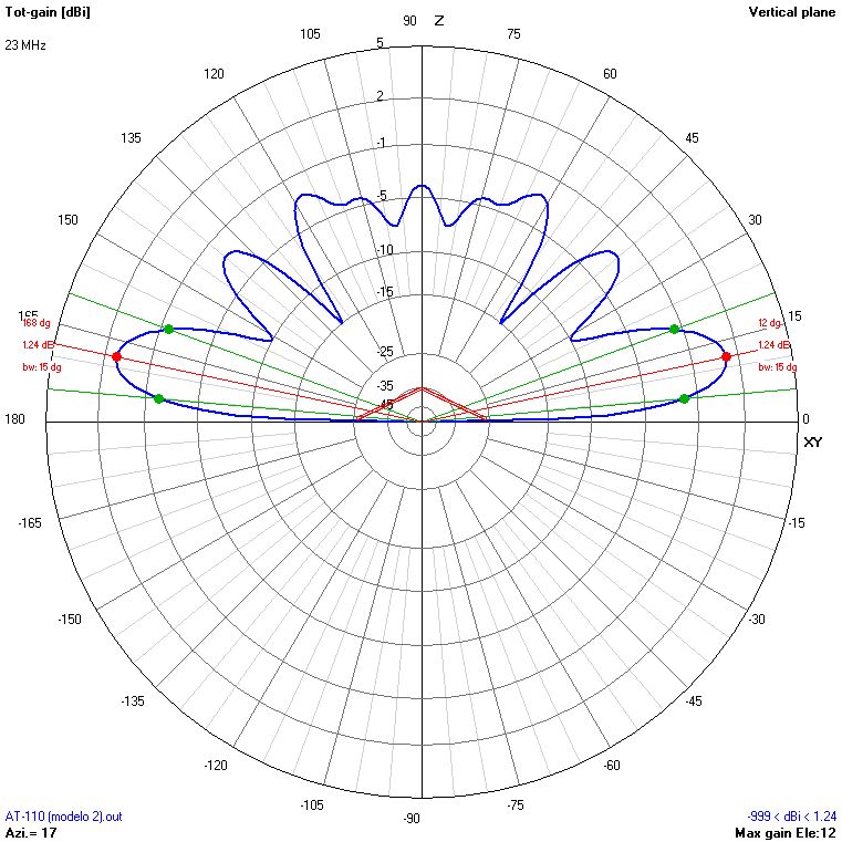
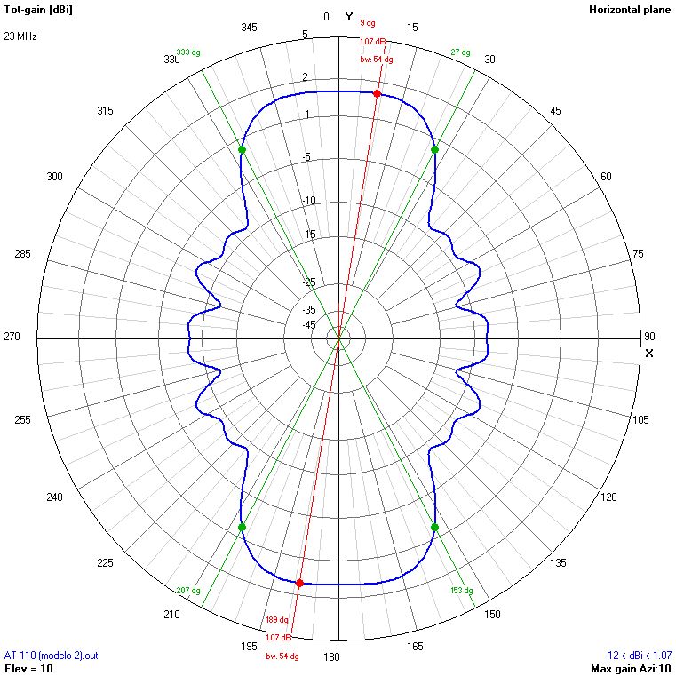
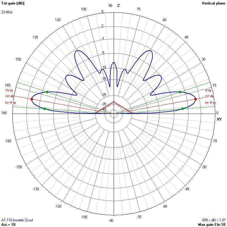
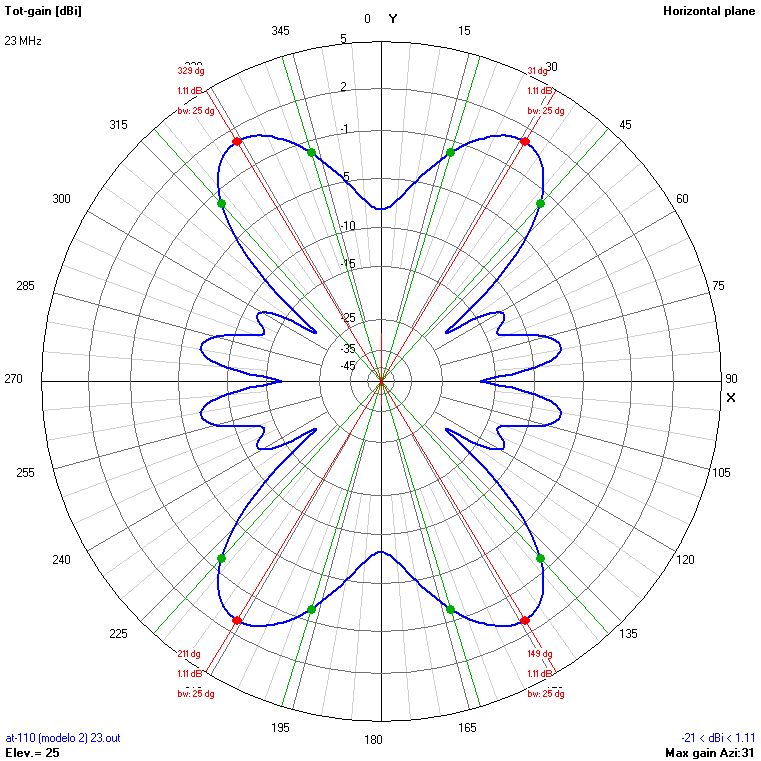
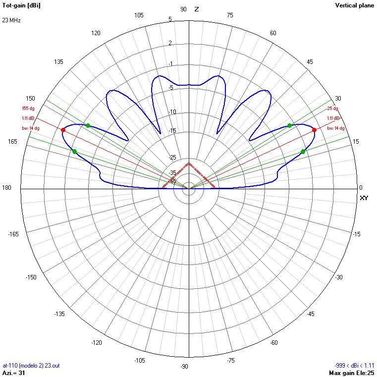
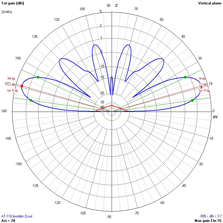
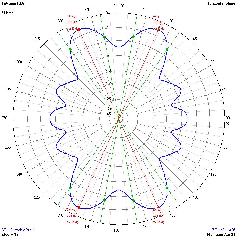
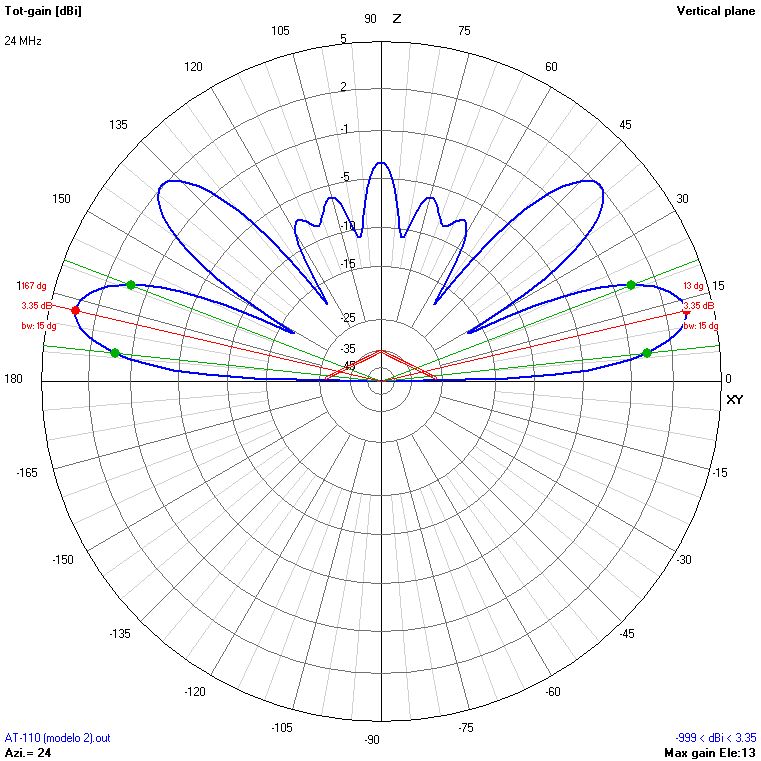
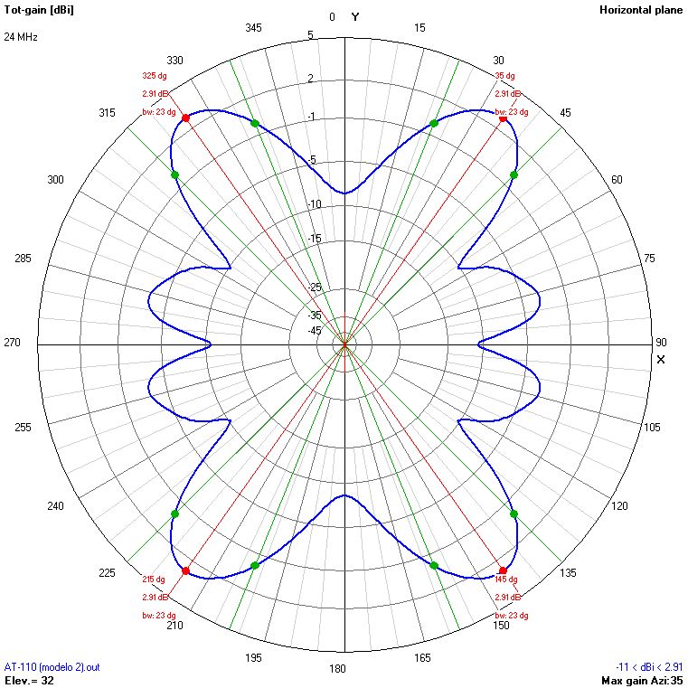
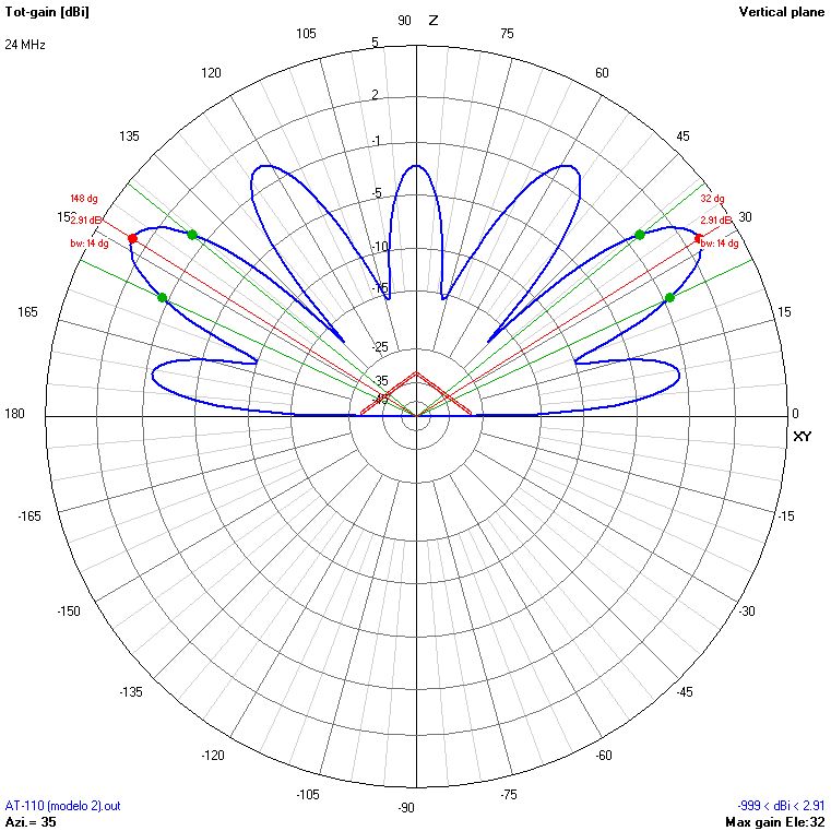
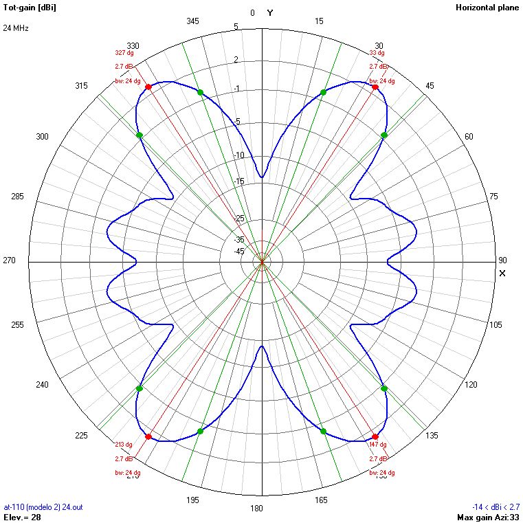
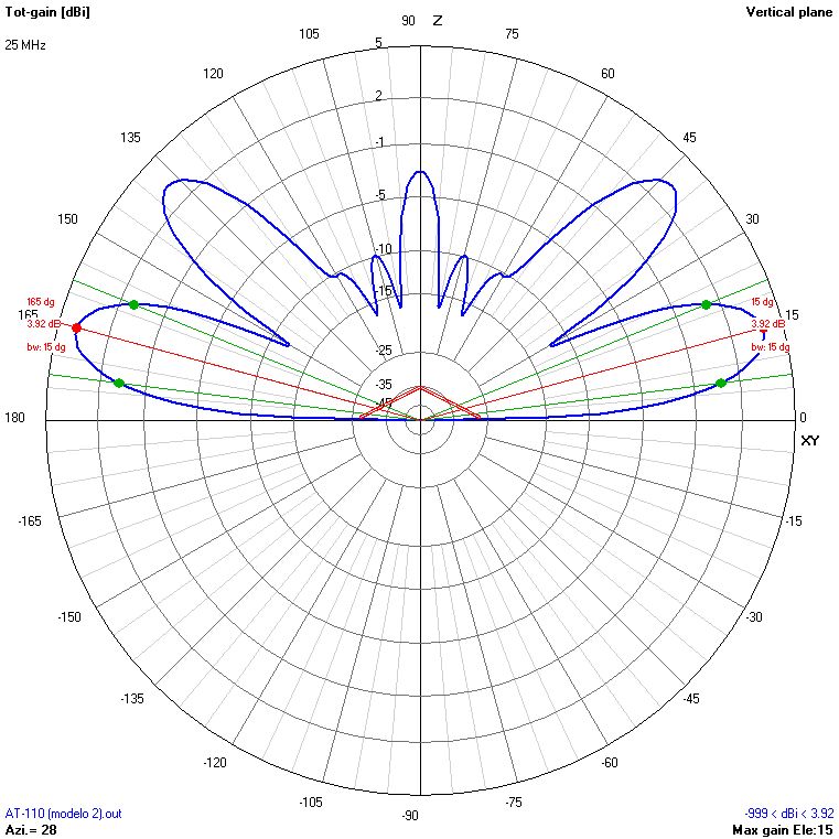
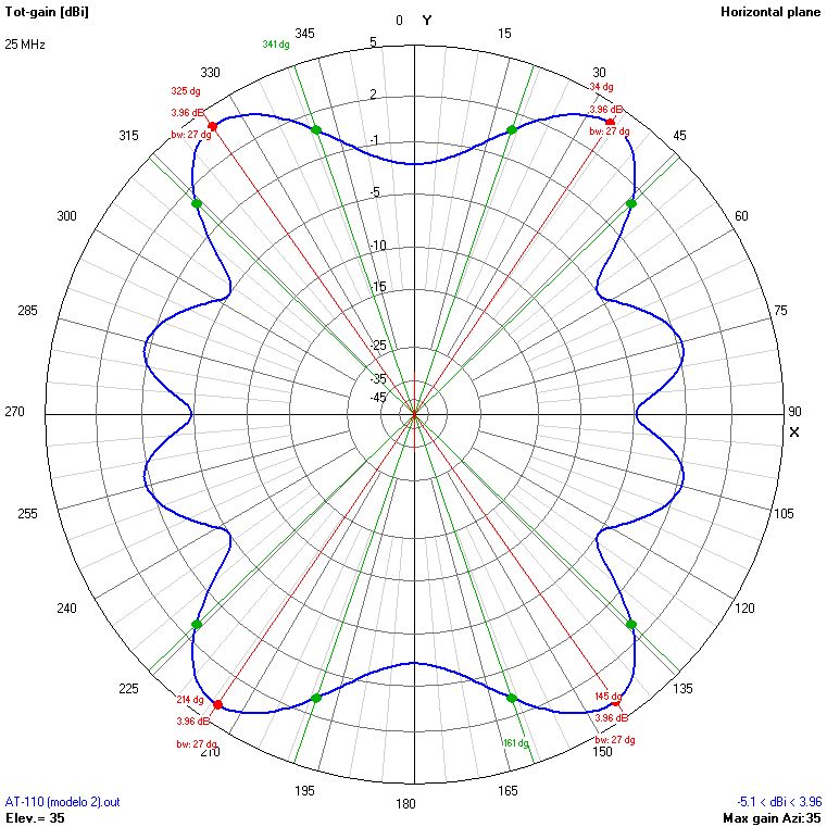
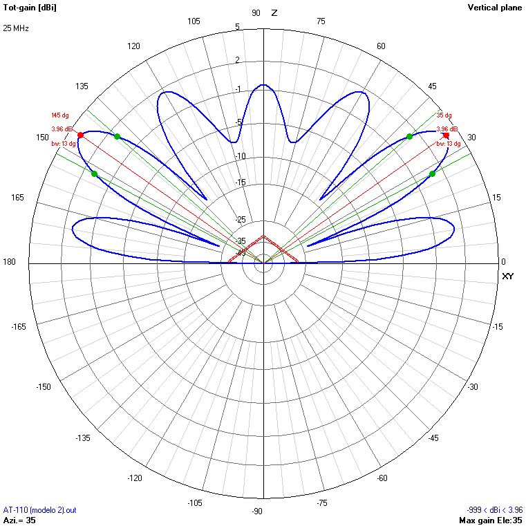
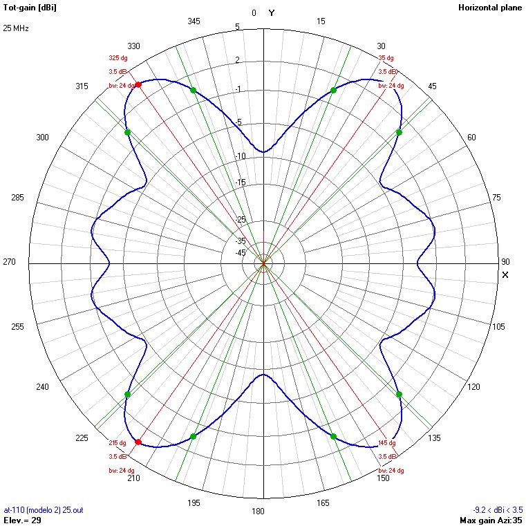
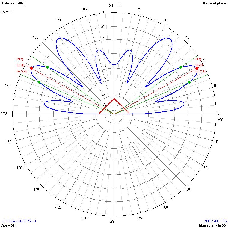
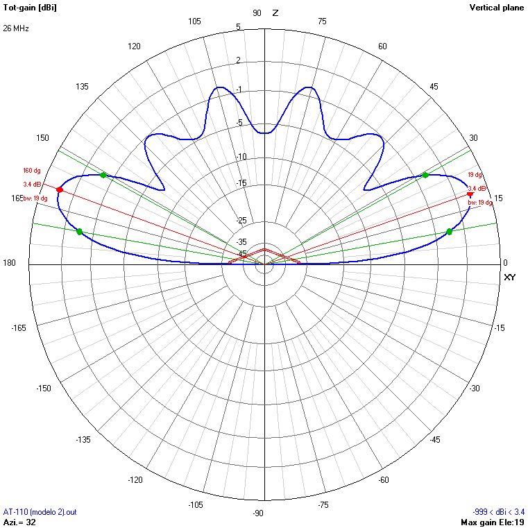
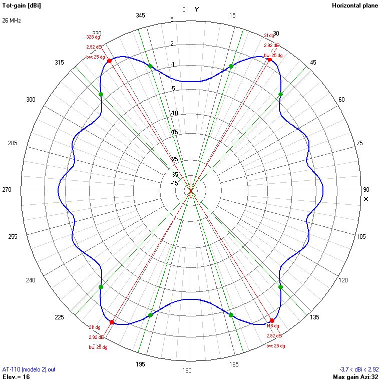
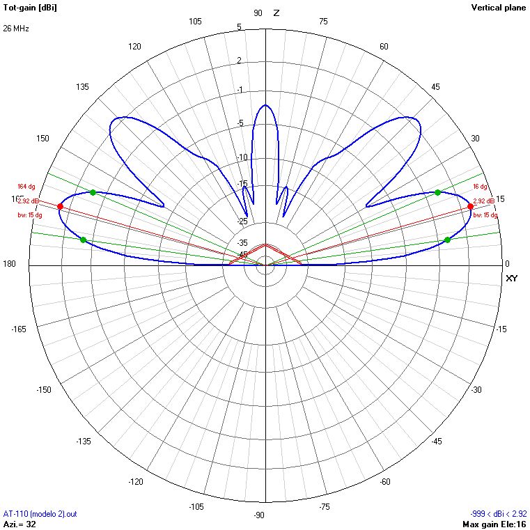
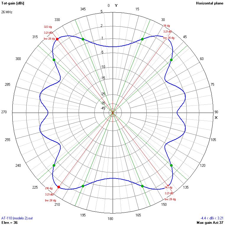
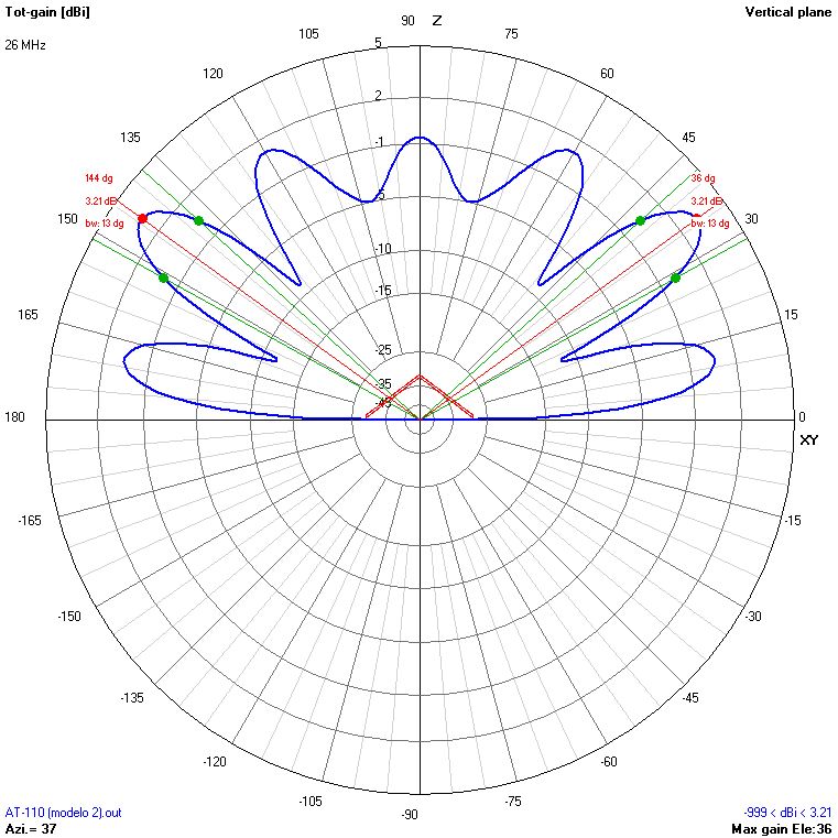
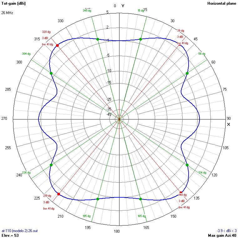
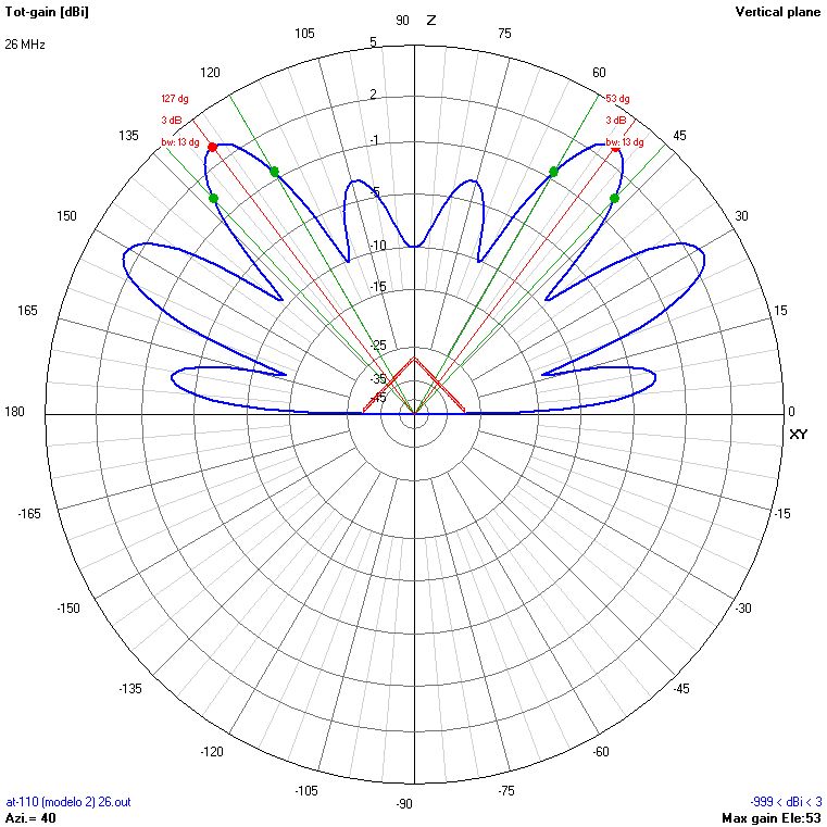
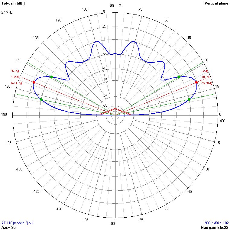
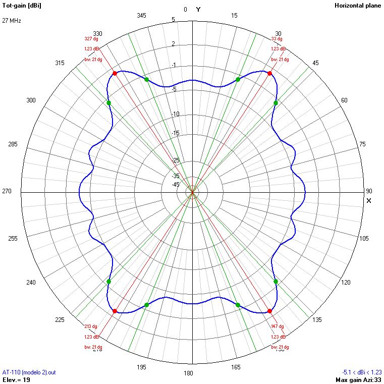
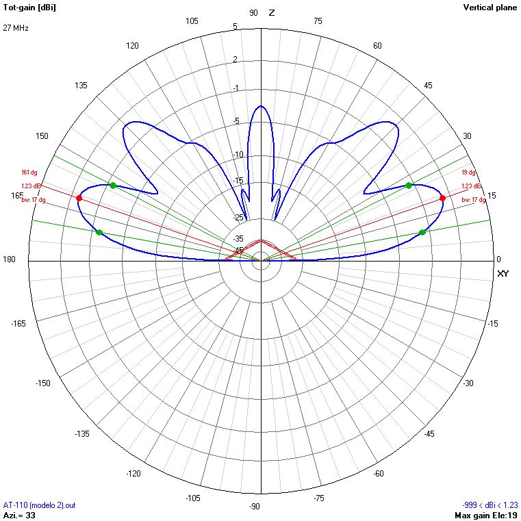
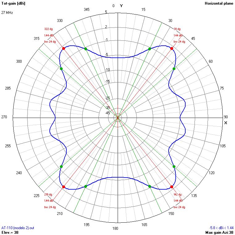
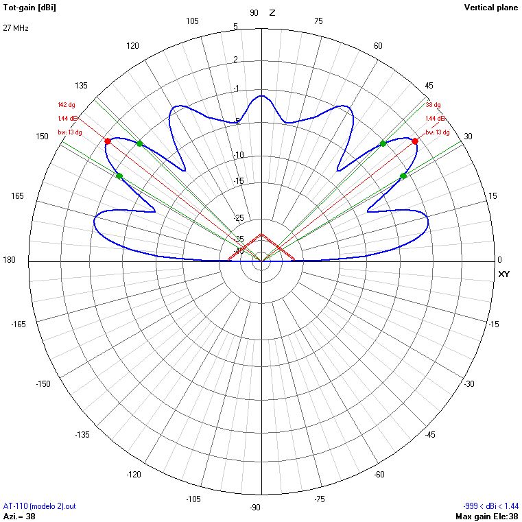
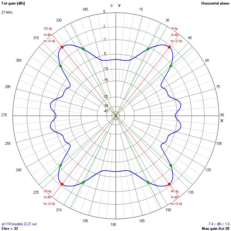
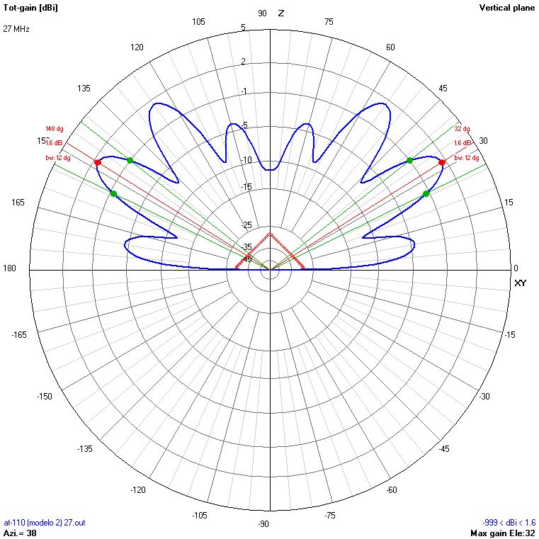
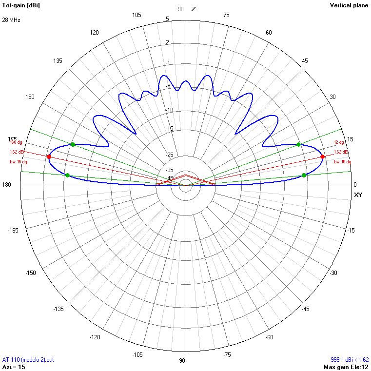
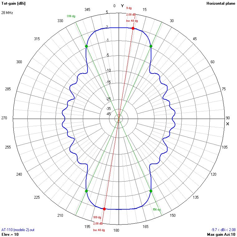
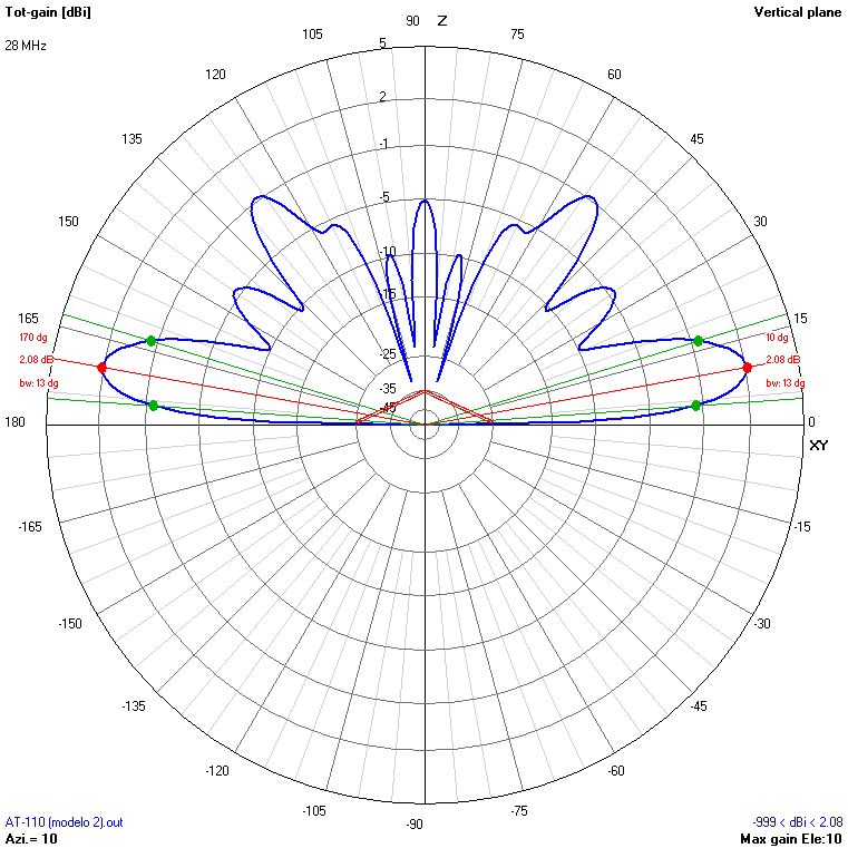
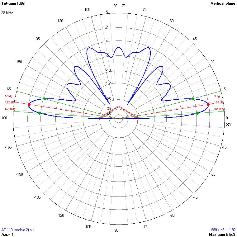
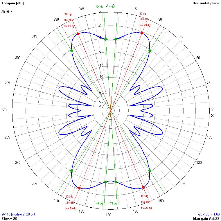
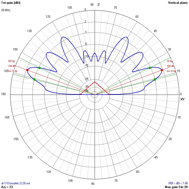
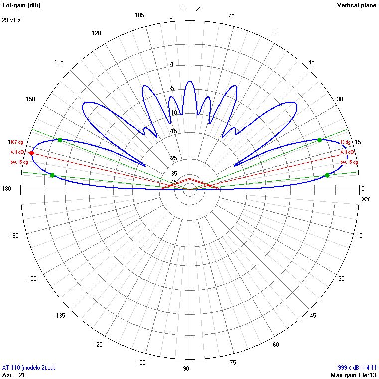
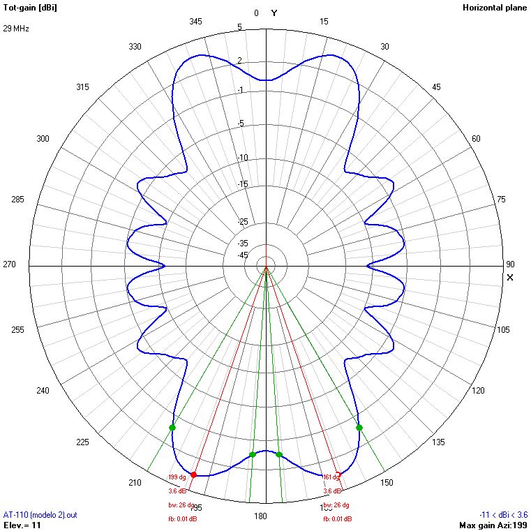
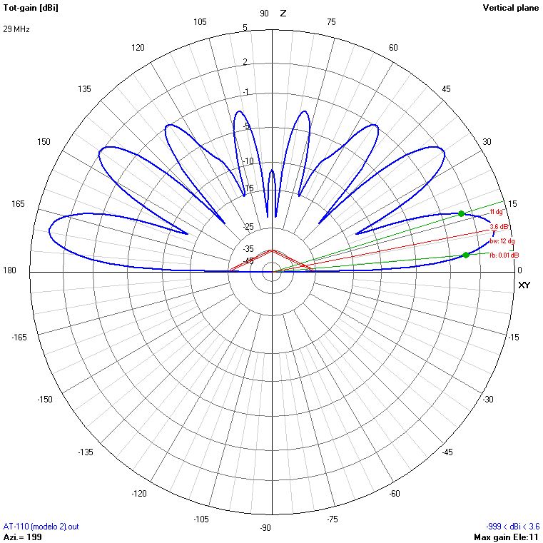
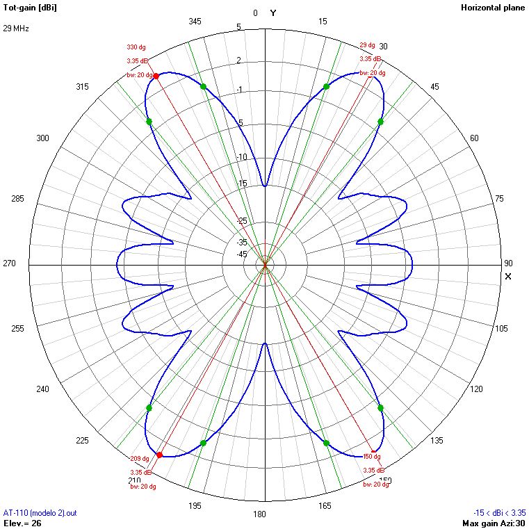
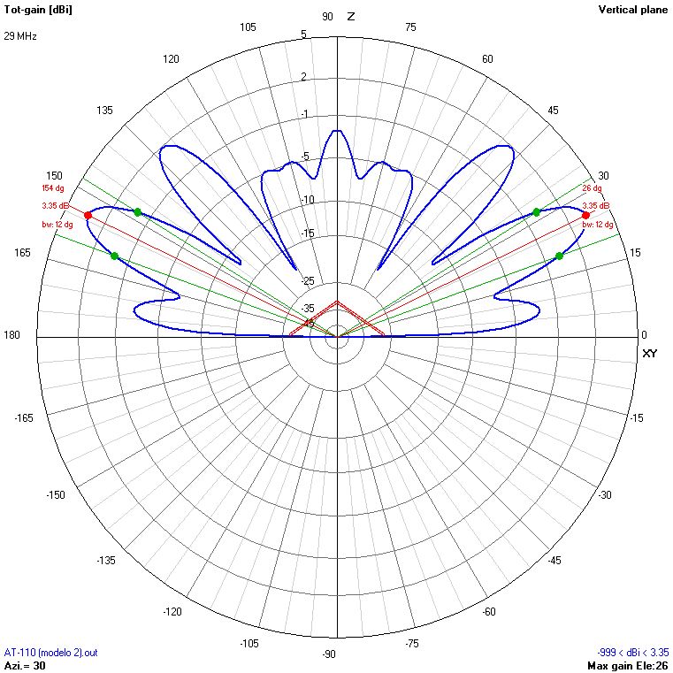
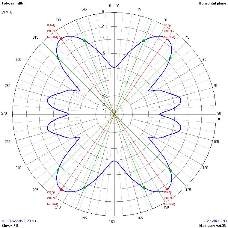
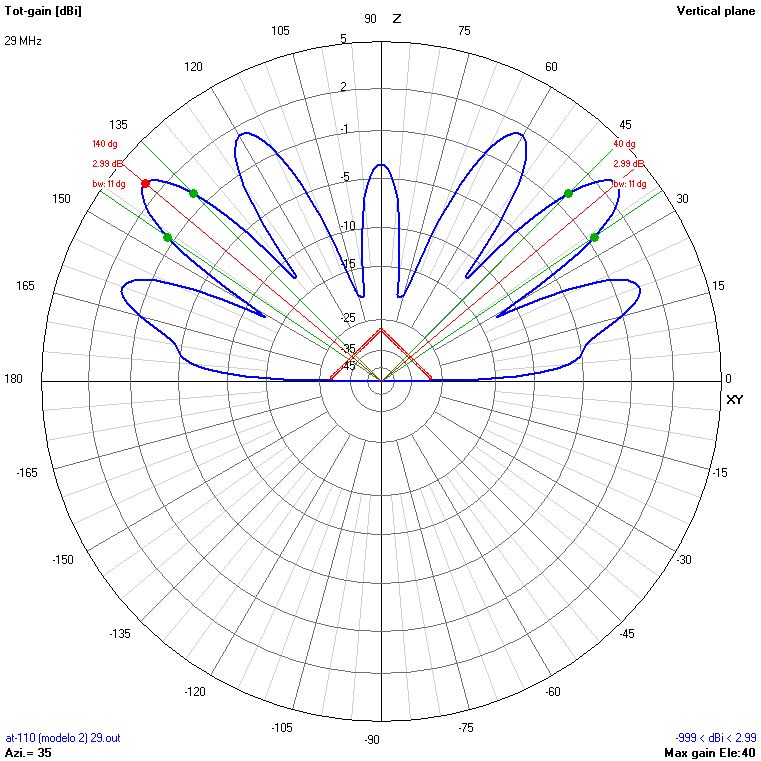
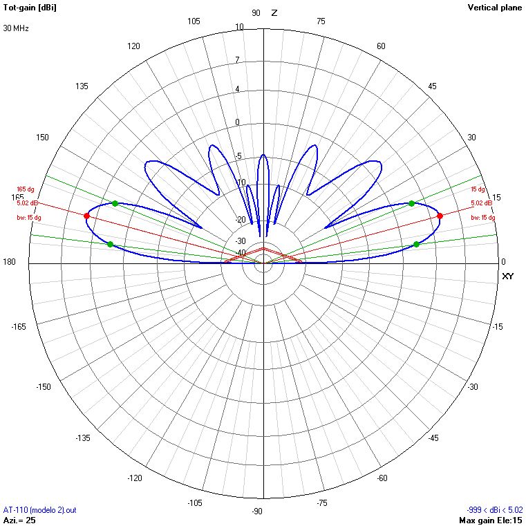
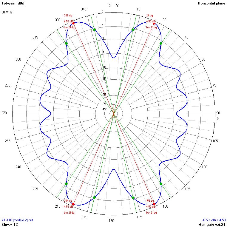
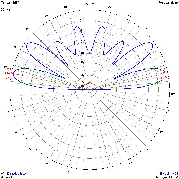
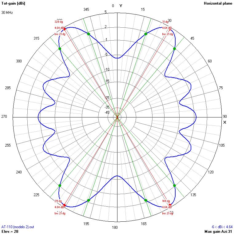
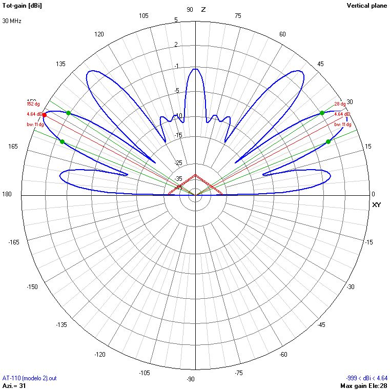
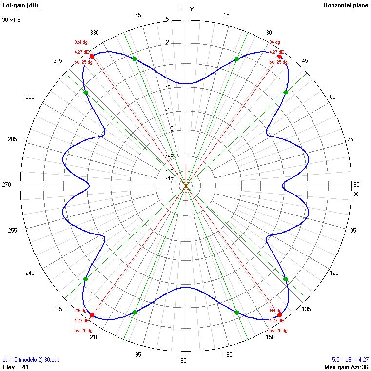
All the radiation patterns shown correspond to the planes of maximum radiation for each frequency. In the case of the vertical patterns, the angle of the azimuth plane where the cut has been made is shown. The same way, in the case of the horizontal patterns, the angle of the elevation plane where the cut has been made is shown. In all the cases, the antenna's position is sketched in red. Please take those considerations into account when comparing patterns of different frequencies.
Remember that in all the simulations, the azimuth is the horizontal angle with respect to the antenna (measured from the Y axis towards the X axis, clockwise). The elevation is the vertical angle with respect to the ground (measured from the Y axis towards the Z axis). Fig. 2 shows a diagram explaining the reference system used.
This way, the antenna is always placed in the plane of azimuth 0º, being 90º the direction perpendicular to the antenna, towards the front. The 90º angle of elevation corresponds to the direction perpendicular to the ground (NVIS).
I will provide also a set of plots of maximum gain for each configuration of installation, indicating the values of azimuth and elevation where the maximum gain occurs. Those plots may be useful to point the antenna at the intended receiver on the other side of the radio link.
For each case, click on the image to see a larger version. The results will be discussed on the section 7.
The table 7 shows the radiation patterns corresponding to the installation of the antenna using masts of 9, 12, 15 and 18 metres.
| Frequency (MHz) | HM=9 α=72,32º | HM=12 α=65,75º | HM=15 α=58,81º | HM=18 α=51,31º | ||||
|---|---|---|---|---|---|---|---|---|
| H | V | H | V | H | V | H | V | |
| 2 | 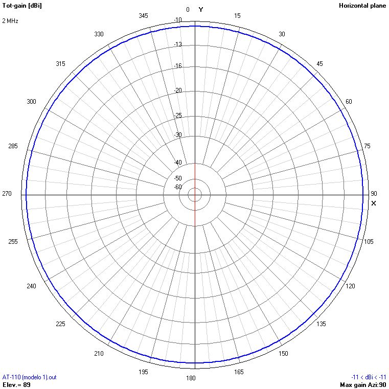 |
 |
 |
 |
 |
 |
 |
 |
| 3 | 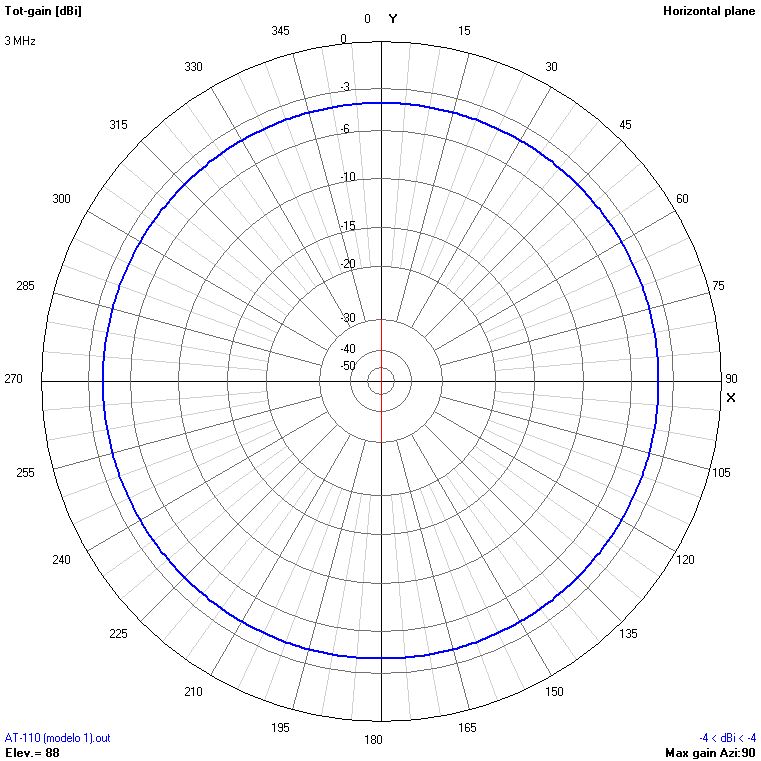 |
 |
 |
 |
 |
 |
 |
 |
| 4 | 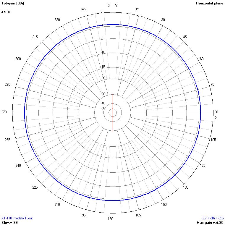 |
 |
 |
 |
 |
 |
 |
 |
| 5 | 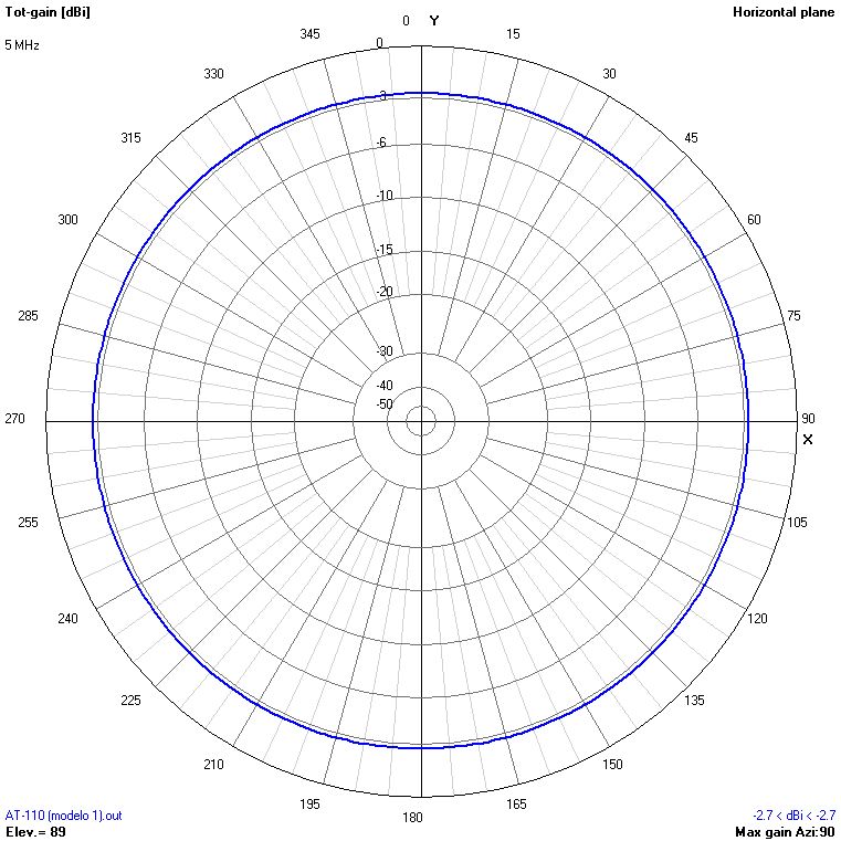 |
 |
 |
 |
 |
 |
 |
 |
| 6 | 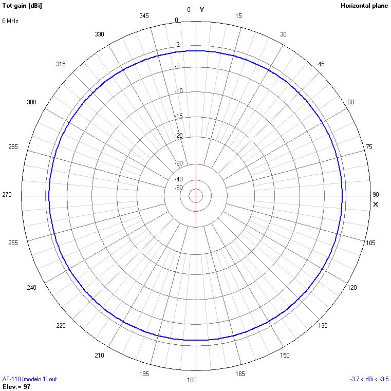 |
 |
 |
 |
 |
 |
 |
 |
| 7 | 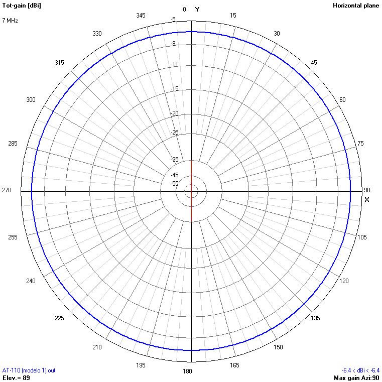 |
 |
 |
 |
 |
 |
 |
 |
| 8 | 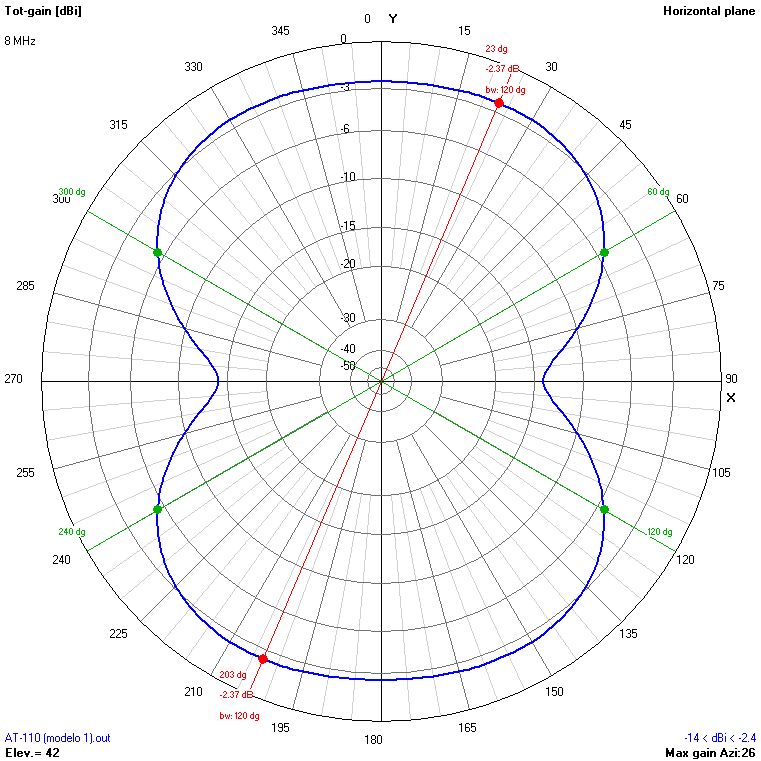 |
 |
 |
 |
 |
 |
 |
 |
| 9 | 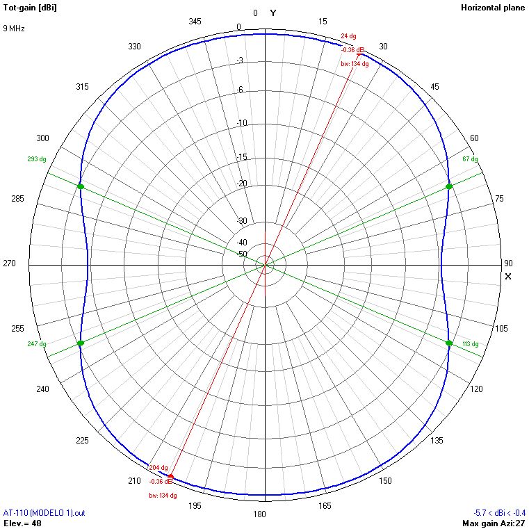 |
 |
 |
 |
 |
 |
 |
 |
| 10 | 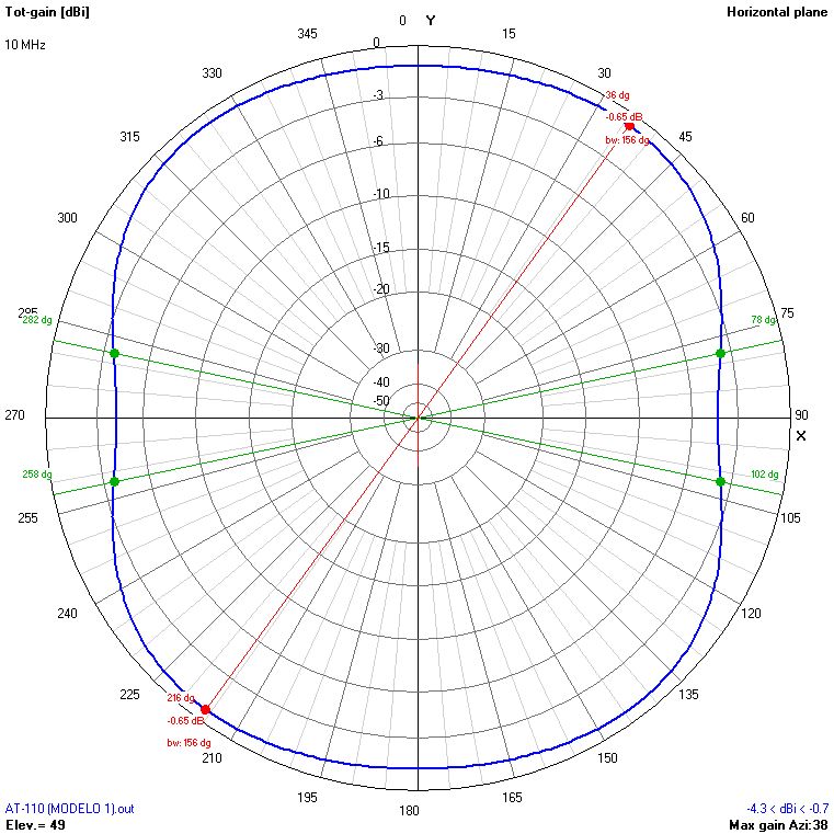 |
 |
 |
 |
 |
 |
 |
 |
| 11 |  |
 |
 |
 |
 |
 |
 |
 |
| 12 | 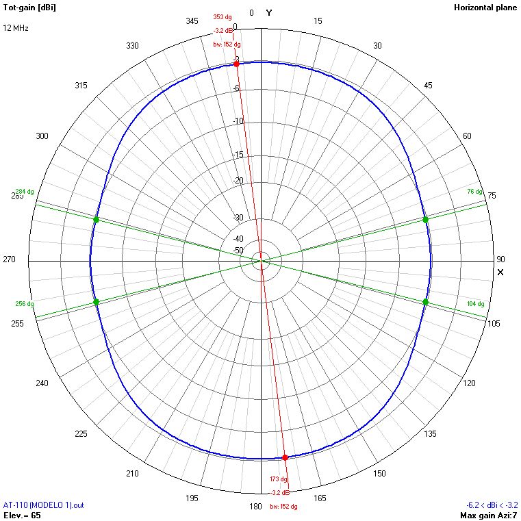 |
 |
 |
 |
 |
 |
 |
 |
| 13 | 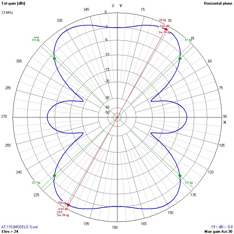 |
 |
 |
 |
 |
 |
 |
 |
| 14 | 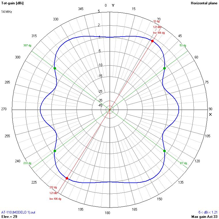 |
 |
 |
 |
 |
 |
 |
 |
| 15 | 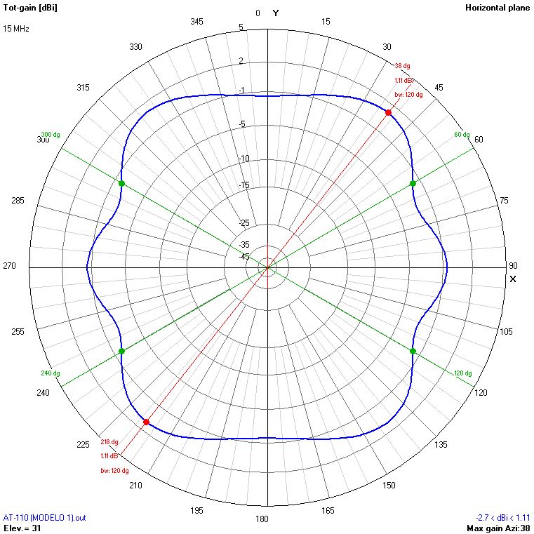 |
 |
 |
 |
 |
 |
 |
 |
| 16 | 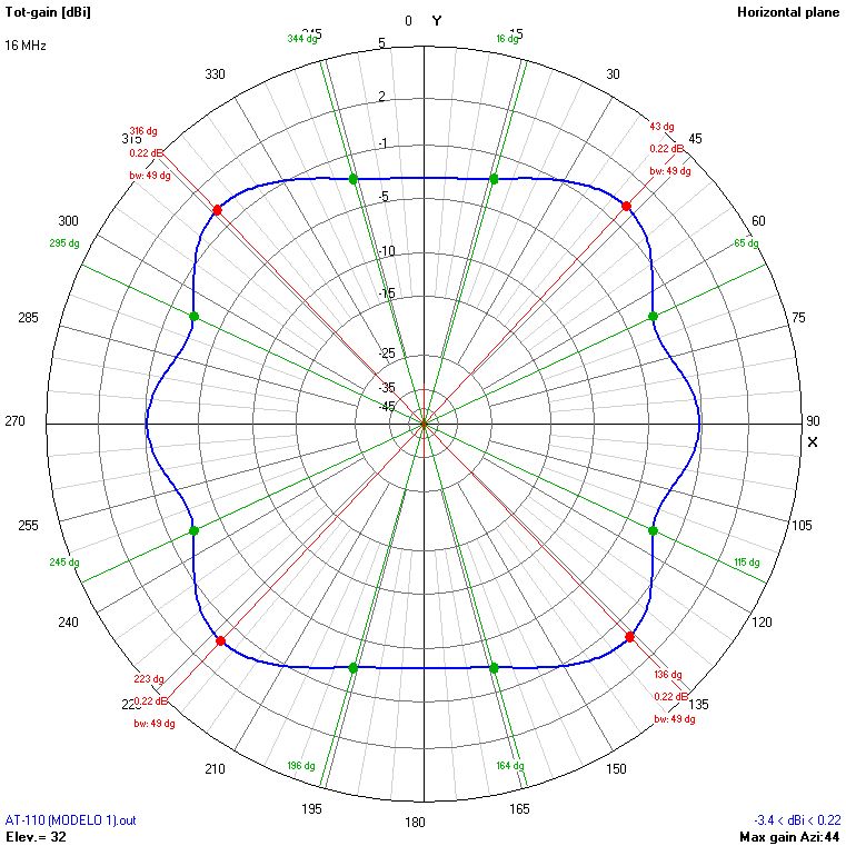 |
 |
 |
 |
 |
 |
 |
 |
| 17 | 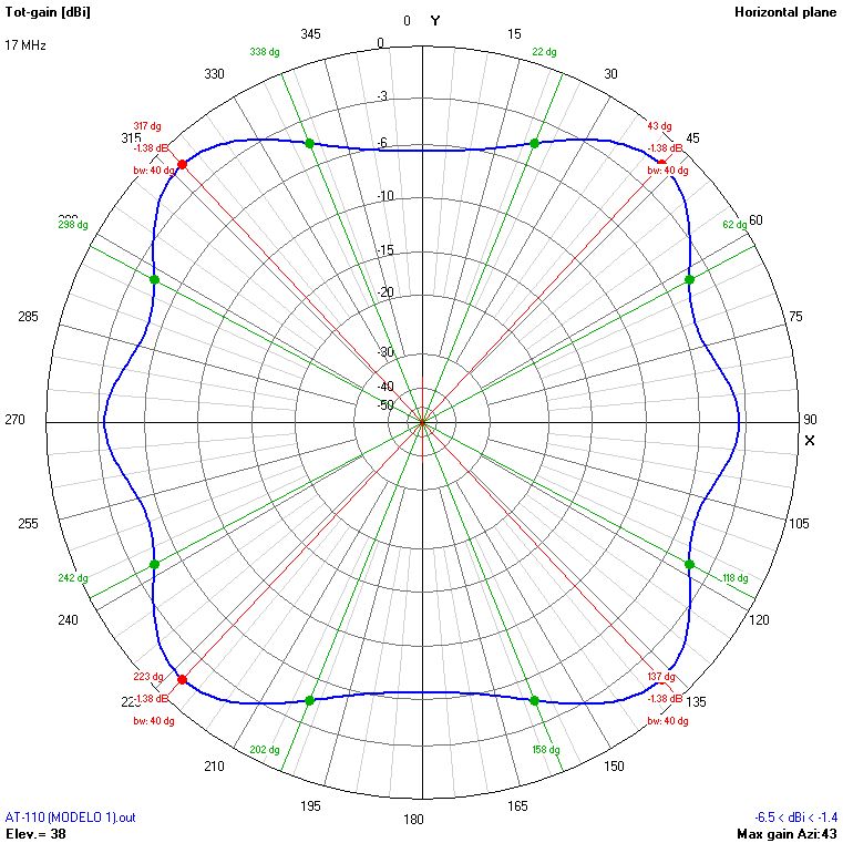 |
 |
 |
 |
 |
 |
 |
 |
| 18 |  |
 |
 |
 |
 |
 |
 |
 |
| 19 | 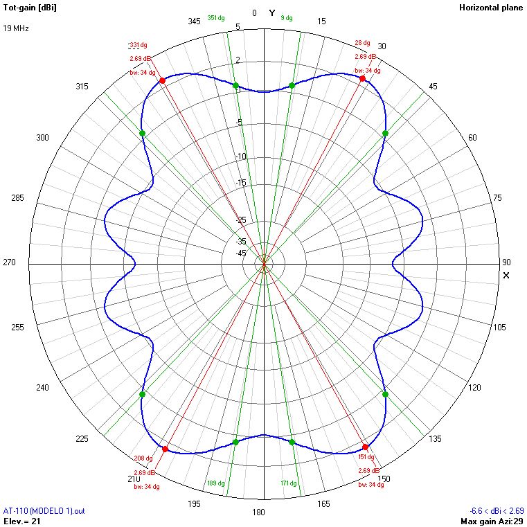 |
 |
 |
 |
 |
 |
 |
 |
| 20 | 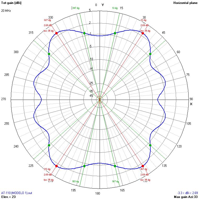 |
 |
 |
 |
 |
 |
 |
 |
| 21 | 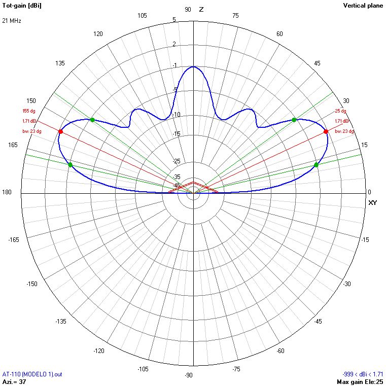 |
 |
 |
 |
 |
 |
 |
 |
| 22 |  |
 |
 |
 |
 |
 |
 |
 |
| 23 | 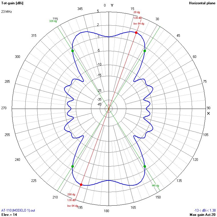 |
 |
 |
 |
 |
 |
 |
 |
| 24 | 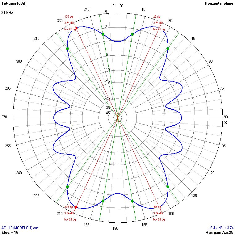 |
 |
 |
 |
 |
 |
 |
 |
| 25 | 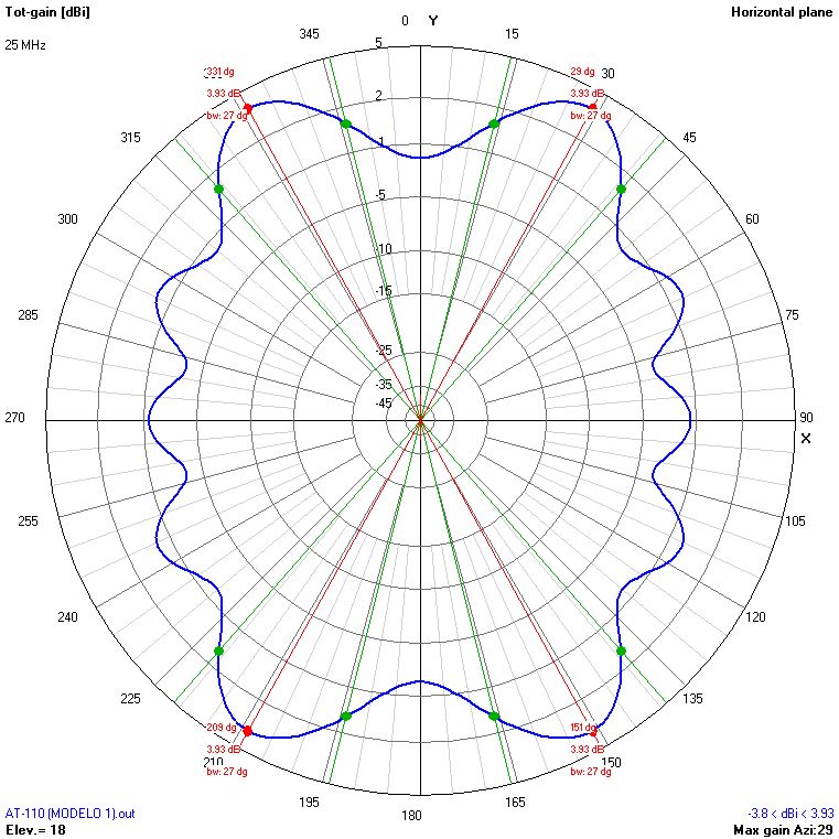 |
 |
 |
 |
 |
 |
 |
 |
| 26 | 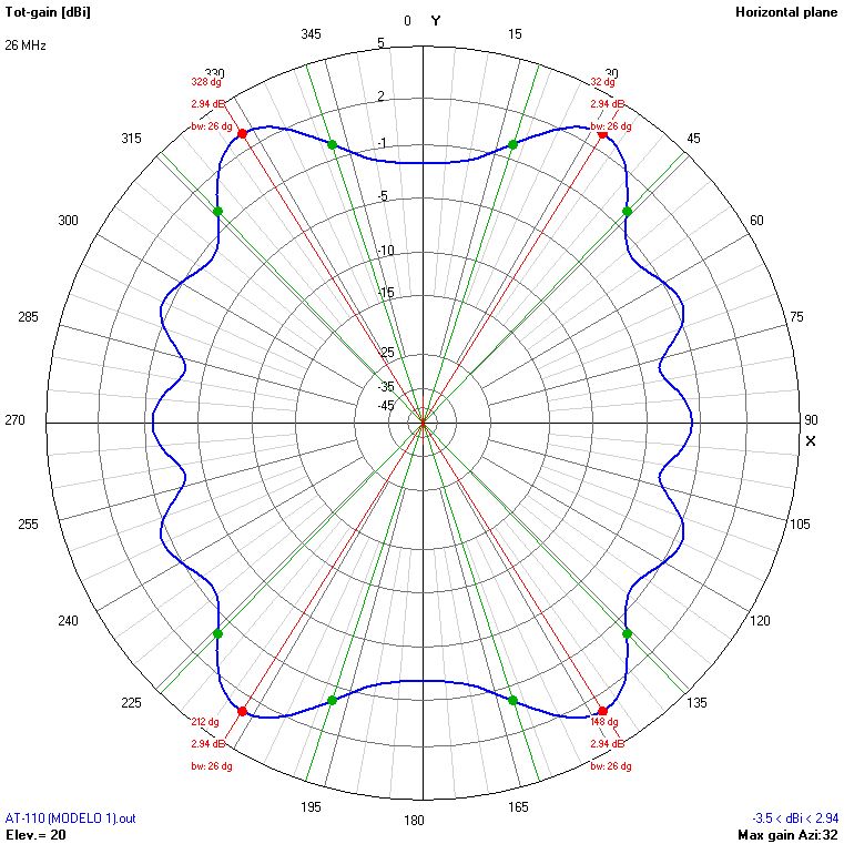 |
 |
 |
 |
 |
 |
 |
 |
| 27 |  |
 |
 |
 |
 |
 |
 |
 |
| 28 | 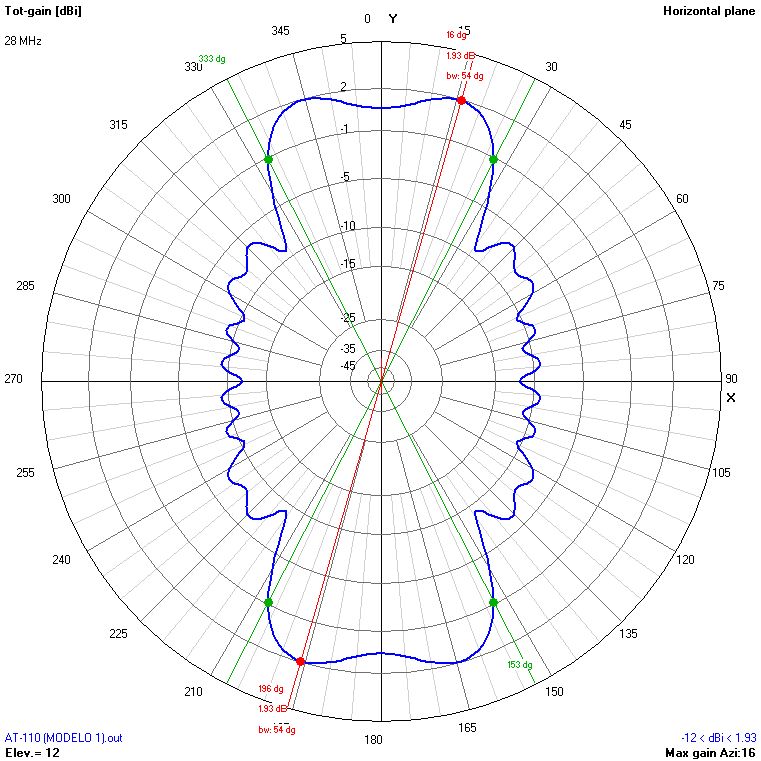 |
 |
 |
 |
 |
 |
 |
 |
| 29 | 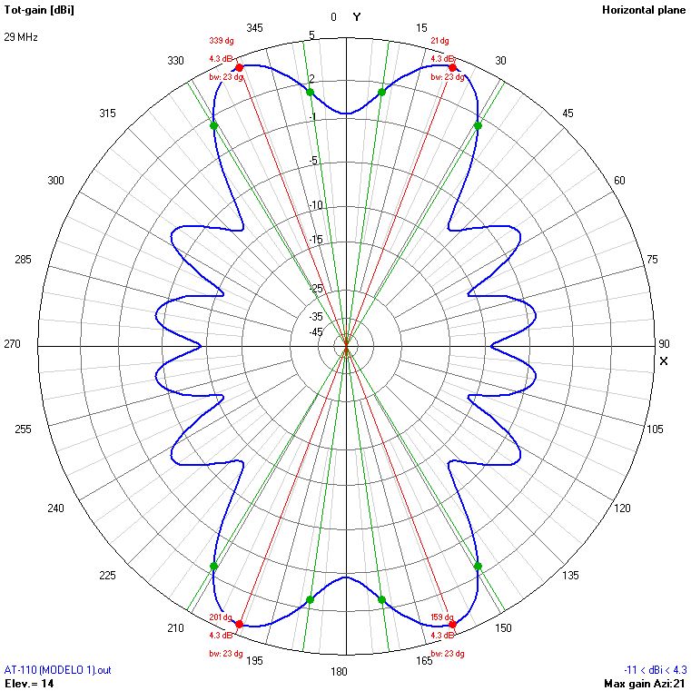 |
 |
 |
 |
 |
 |
 |
 |
| 30 | 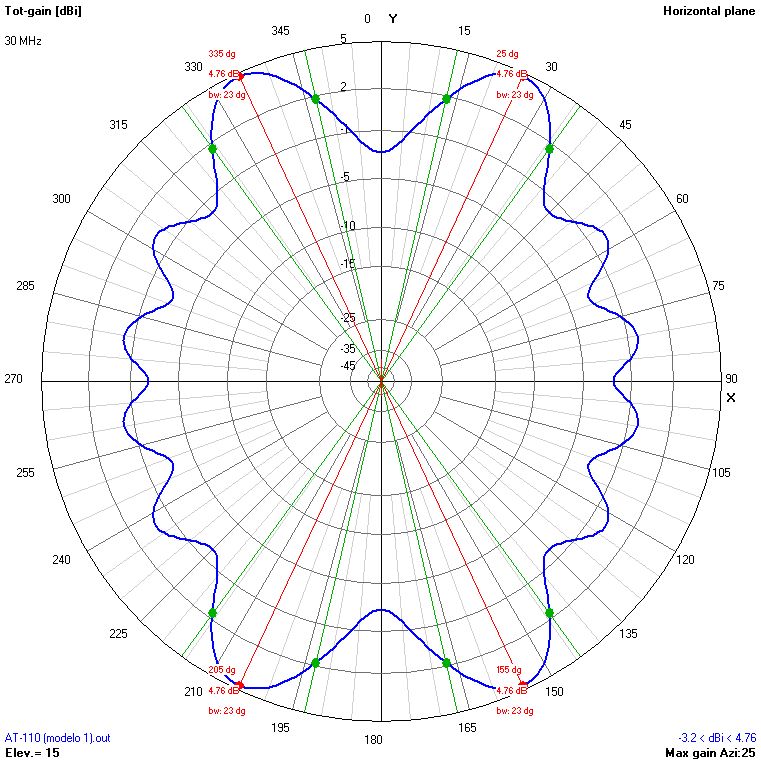 |
 |
 |
 |
 |
 |
 |
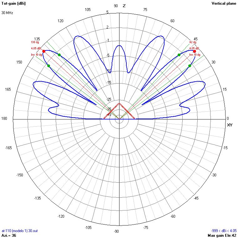 |
Table 7. Radiation patterns of the AT-110A antenna using masts of 9, 12, 15 and 18 metres. Simulation model 1.
Below you will find the plots of maximum gain using masts of 9, 12, 15 and 18 metres. Click on each image to see a larger version.
The figure 6 shows the plot of maximum gain for a height of installation HM = 9 metres.
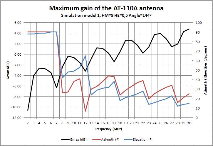
Fig. 6. Maximum gain of the AT-110A antenna with a mast of 9 metres. Simulation model 1.
The figure 7 shows the plot of maximum gain for a height of installation HM = 12 metres.
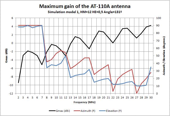
Fig. 7. Maximum gain of the AT-110A antenna with a mast of 12 metres. Simulation model 1.
The figure 8 shows the plot of maximum gain for a height of installation HM = 15 metres.
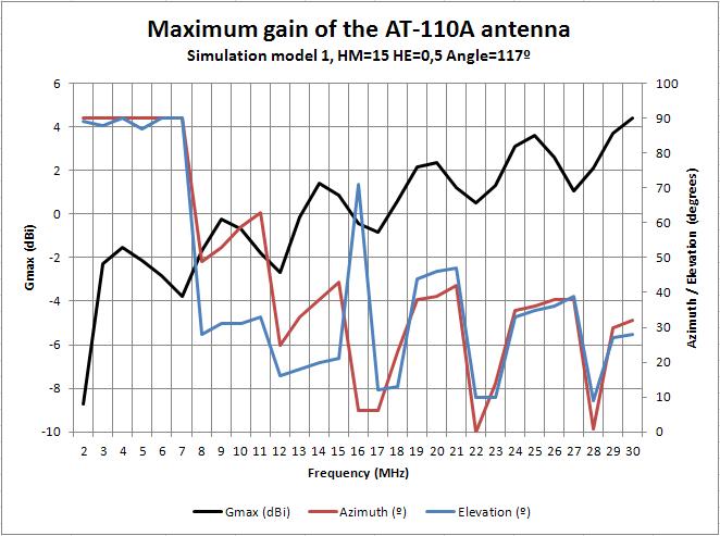
Fig. 8. Maximum gain of the AT-110A antenna with a mast of 15 metres. Simulation model 1.
The figure 9 shows the plot of maximum gain for a height of installation HM = 18 metres.
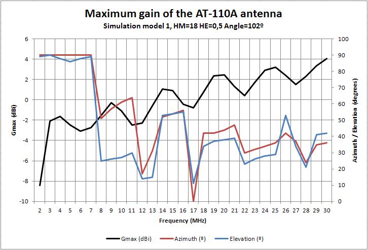
Fig. 9 Maximum gain of the AT-110A antenna with a mast of 18 metres. Simulation model 1.
Finally, the figure 10 shows a comparison of the maximum gain for the four installation configurations analysed.
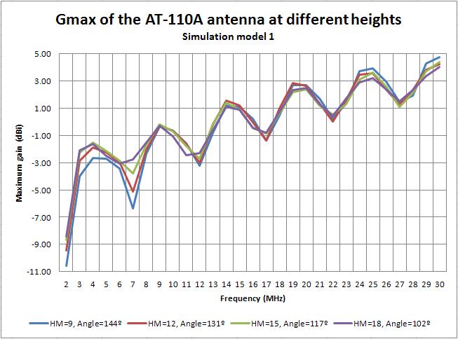
Fig. 10. Comparison of the maximum gain of the AT-110A antenna with different masts. Simulation model 1.
The results will be analysed on the section 7.
6. Simulation of the AT-110A antenna (model 2).
6. Simulation of the AT-110A antenna (model 2).
In this section I will show the results of the simulations performed with the Invelco AT-110A antenna 4NEC2 model 2, presented in the section 2. The values of L, S, R and φ can be consulted in the antenna's user manual.
In all the simulations, a ground of average type is considered, with a conductivity of 0.005 S/m and a dielectric constant of 13.
I have used discrete frequencies in all the working range of the antenna (2-30 MHz), at 1 MHz intervals or even at 200 kHz intervals when necessary.
On the other hand, the SWR calculations will be referred to a characteristic impedance of 450 ohms (9:1 balun in order to work with 50 ohms radios).
I have simulated configurations with masts of lengths HM equal to 9 m, 12 m, 15 m and 18 m, being for all of them the height of installation of the tips HE equal to 0,5 m. In those four cases, the angle between the two legs of the antena will be of 144º, 131º, 117º and 102º, respectively.
Finally, in all the simulations a resolution of 1 degree will be used.
6.1. Computation of the standing wave ratio (SWR).
Fig. 11 shows the SWR vs frequency plots resulting from the simulations of the model 2. Click on the image to see a larger version.
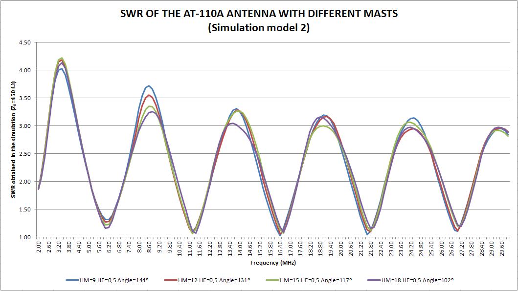
Fig. 11. SWR of the AT-110A antenna with different masts. Simulation model 2.
The results will be analysed in the section 7.
6.2. Simulation of radiation patterns.
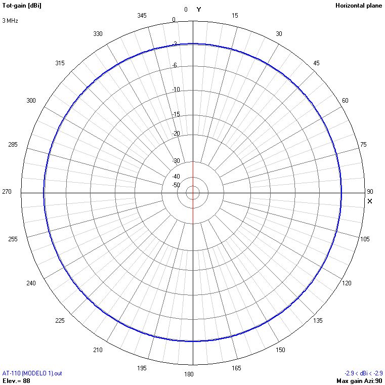
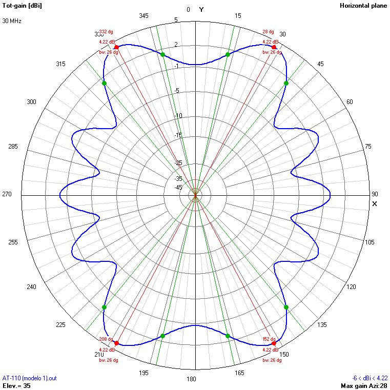
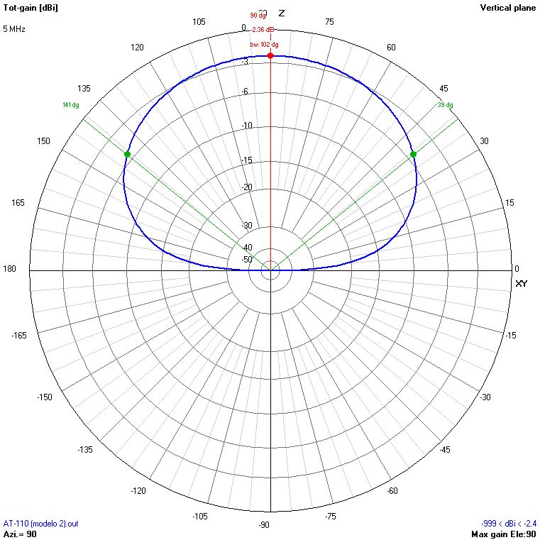
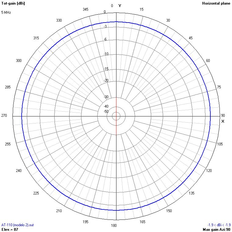
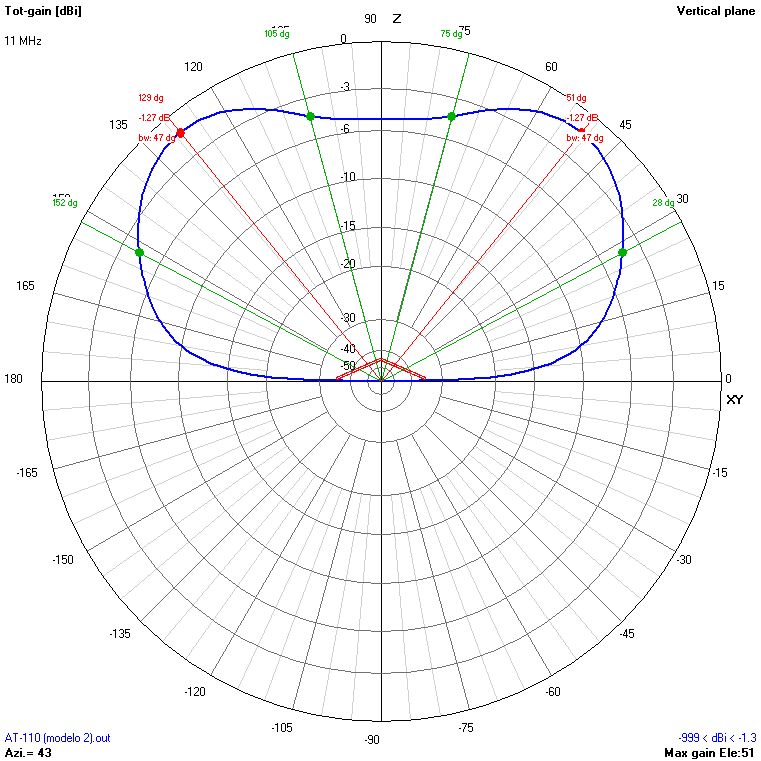
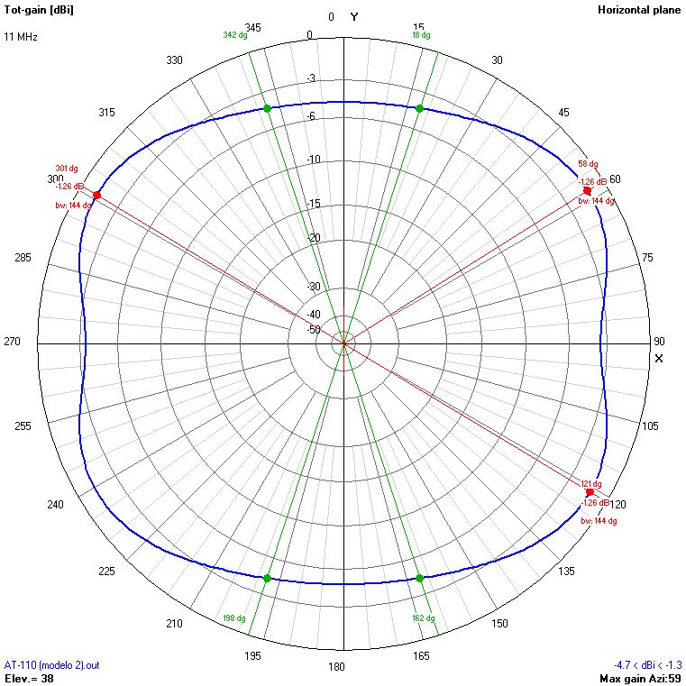
In this section, the results of the simulations of the model 1 are shown (see section 2.2), consisting of radiation patterns for frequencies between 2 MHz and 30 MHz at 1 MHz intervals and for masts of 9, 12, 15 and 18 m. The antenna is installed in inverted-vee configuration with the tips at 0,5 metres over ground.
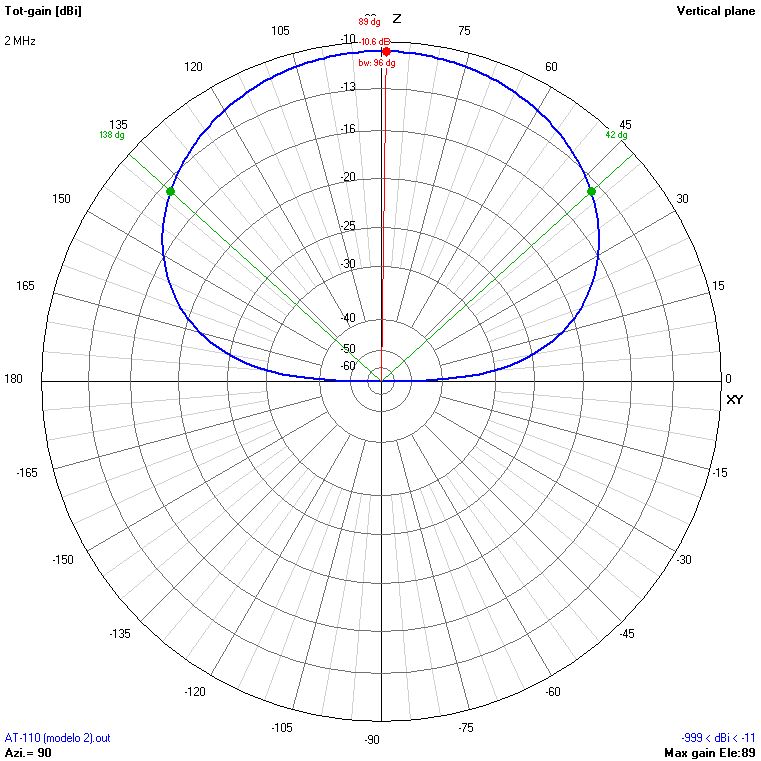
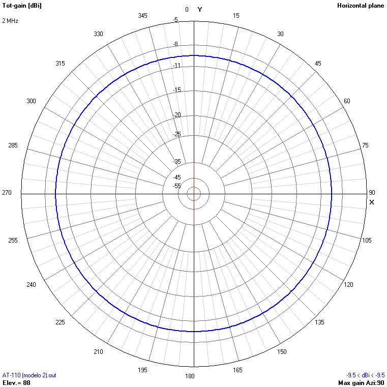
All the radiation patterns shown correspond to the planes of maximum radiation for each frequency. In the case of the vertical patterns, the angle of the azimuth plane where the cut has been made is shown. The same way, in the case of the horizontal patterns, the angle of the elevation plane where the cut has been made is shown. In all the cases, the antenna's position is sketched in red. Please take those considerations into account when comparing patterns of different frequencies.
Remember that in all the simulations, the azimuth is the horizontal angle with respect to the antenna (measured from the Y axis towards the X axis, clockwise). The elevation is the vertical angle with respect to the ground (measured from the Y axis towards the Z axis). Fig. 2 shows a diagram explaining the reference system used.
This way, the antenna is always placed in the plane of azimuth 0º, being 90º the direction perpendicular to the antenna, towards the front. The 90º angle of elevation corresponds to the direction perpendicular to the ground (NVIS).
I will provide also a set of plots of maximum gain for each configuration of installation, indicating the values of azimuth and elevation where the maximum gain occurs. Those plots may be useful to point the antenna at the intended receiver on the other side of the radio link.
For each case, click on the image to see a larger version. The results will be discussed on the section 7.
The table 8 shows the radiation patterns corresponding to the installation of the antenna using masts of 9, 12, 15 and 18 metres.
| Frequency (MHz) | HM=9 α=72,32º | HM=12 α=65,75º | HM=15 α=58,81º | HM=18 α=51,31º | ||||
|---|---|---|---|---|---|---|---|---|
| H | V | H | V | H | V | H | V | |
| 2 |  |
 |
 |
 |
 |
 |
 |
 |
| 3 | 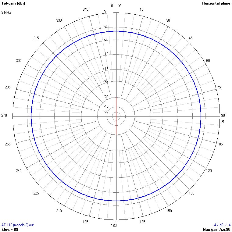 |
 |
 |
 |
 |
 |
 |
 |
| 4 | 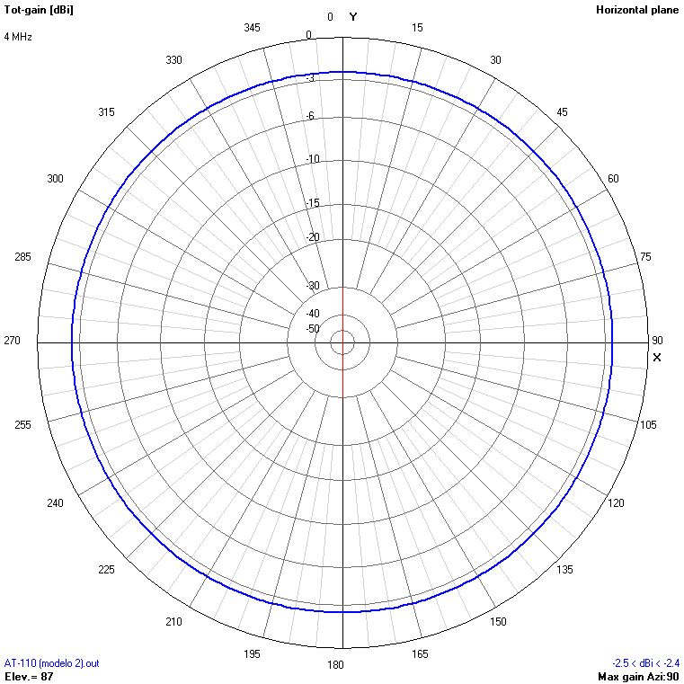 |
 |
 |
 |
 |
 |
 |
 |
| 5 | 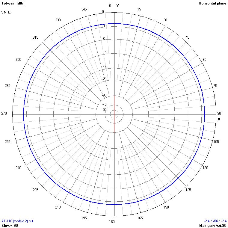 |
 |
 |
 |
 |
 |
 |
 |
| 6 | 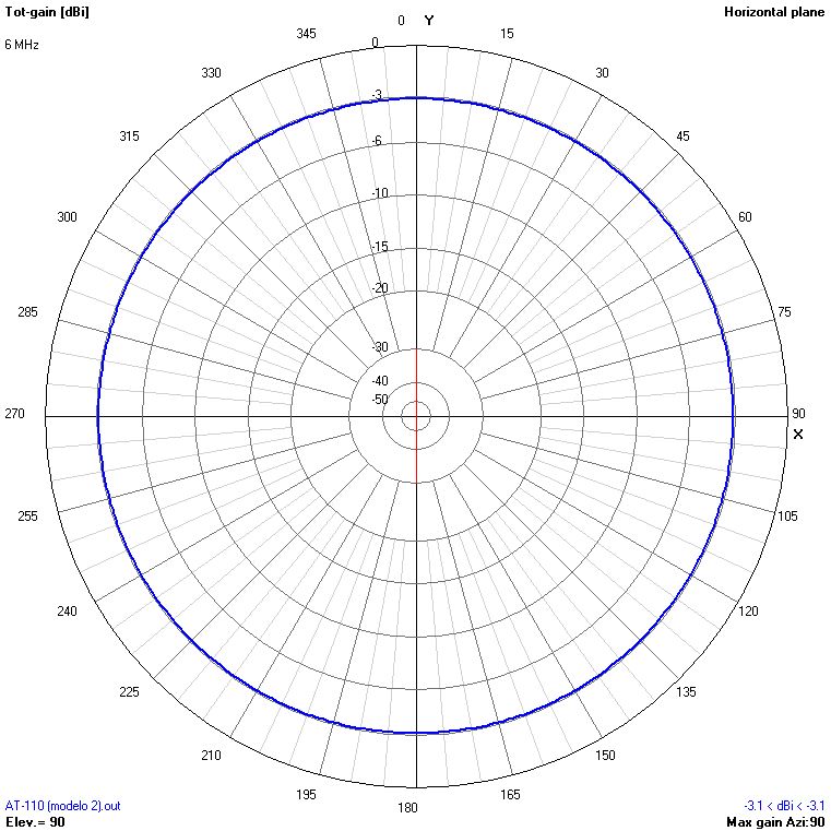 |
 |
 |
 |
 |
 |
 |
 |
| 7 | 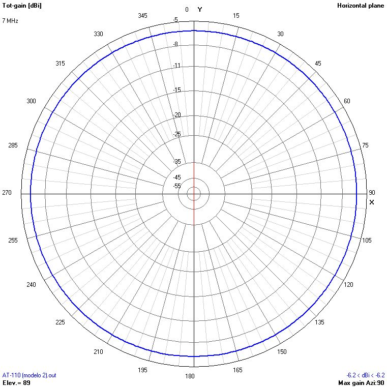 |
 |
 |
 |
 |
 |
 |
 |
| 8 | 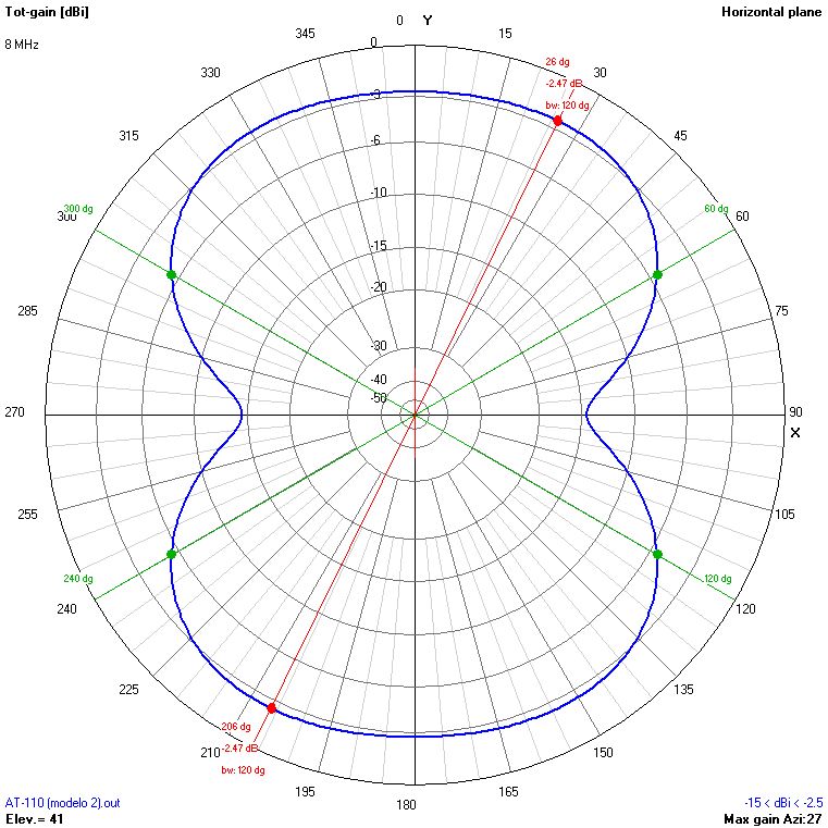 |
 |
 |
 |
 |
 |
 |
 |
| 9 | 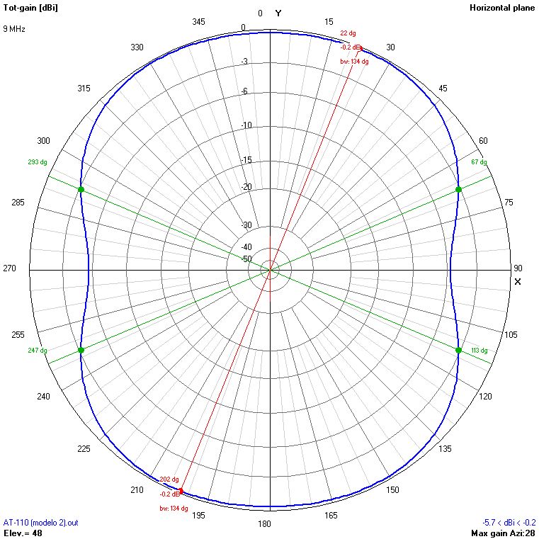 |
 |
 |
 |
 |
 |
 |
 |
| 10 | 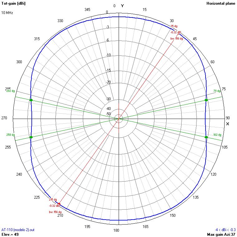 |
 |
 |
 |
 |
 |
 |
 |
| 11 | 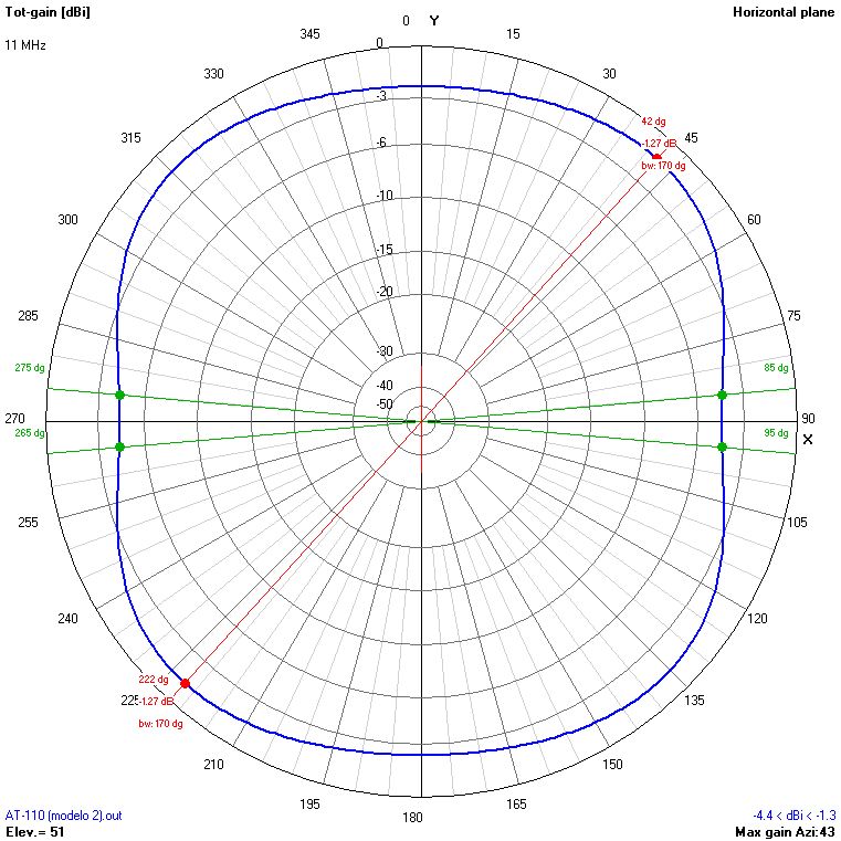 |
 |
 |
 |
 |
 |
 |
 |
| 12 | 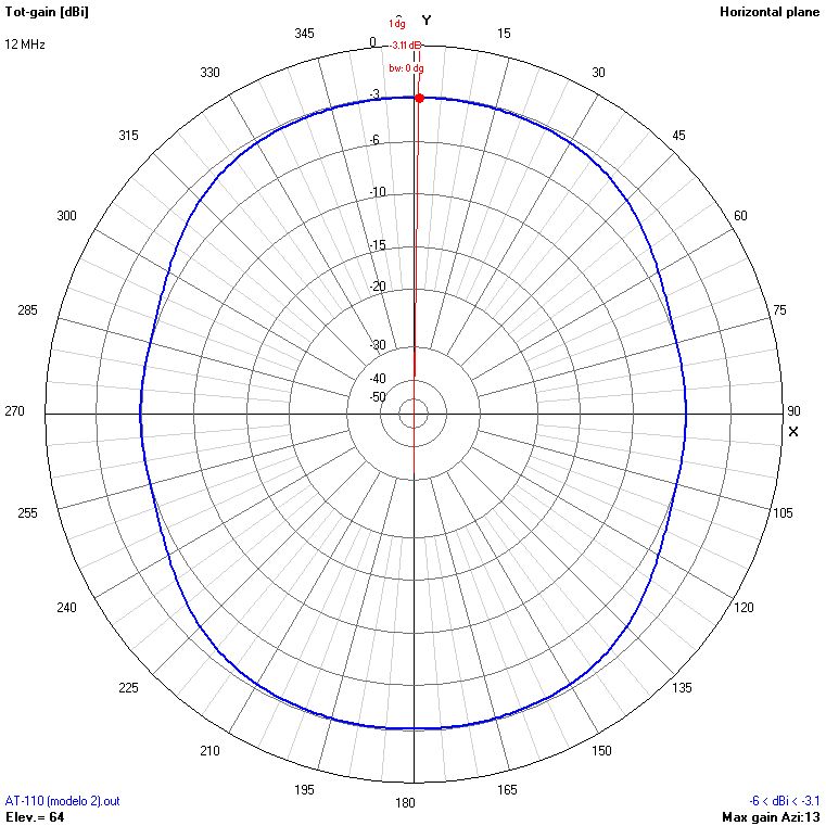 |
 |
 |
 |
 |
 |
 |
 |
| 13 | 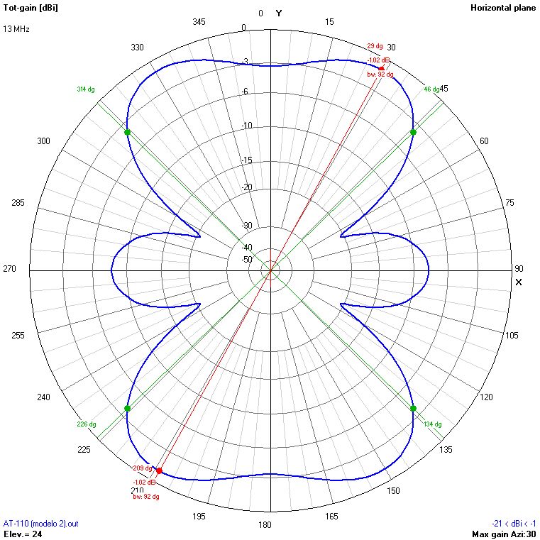 |
 |
 |
 |
 |
 |
 |
 |
| 14 | 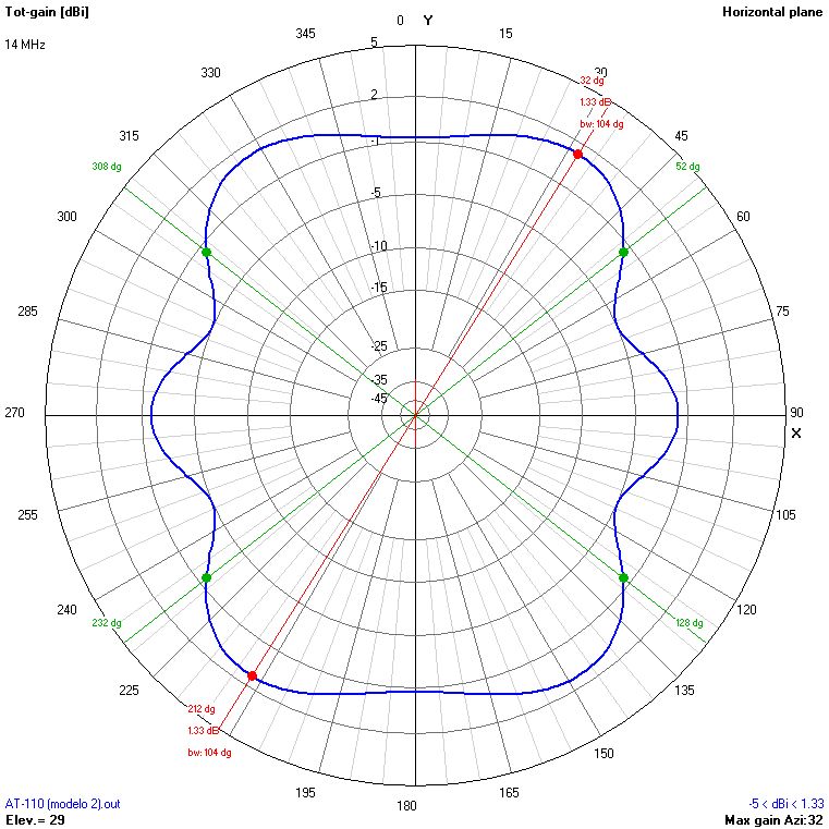 |
 |
 |
 |
 |
 |
 |
 |
| 15 | 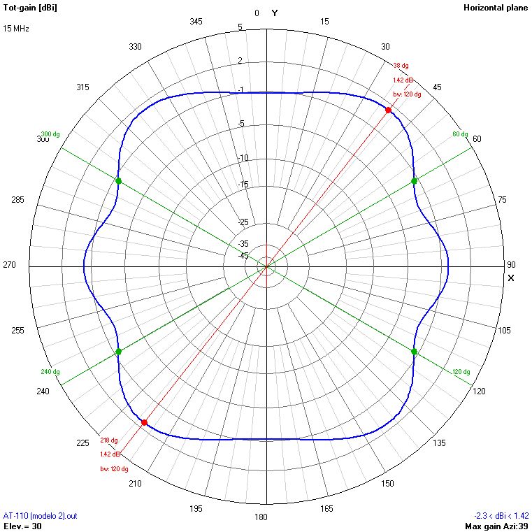 |
 |
 |
 |
 |
 |
 |
 |
| 16 | 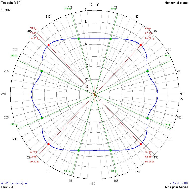 |
 |
 |
 |
 |
 |
 |
 |
| 17 | 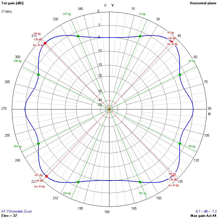 |
 |
 |
 |
 |
 |
 |
 |
| 18 | 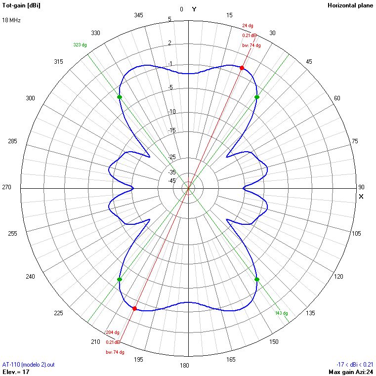 |
 |
 |
 |
 |
 |
 |
 |
| 19 | 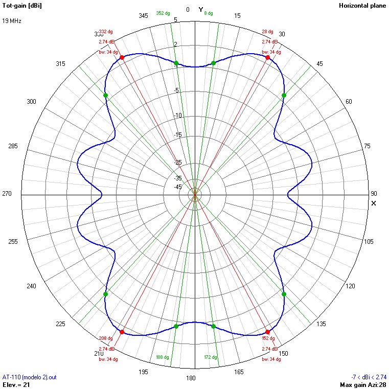 |
 |
 |
 |
 |
 |
 |
 |
| 20 | 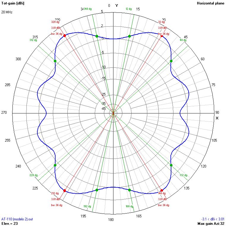 |
 |
 |
 |
 |
 |
 |
 |
| 21 |  |
 |
 |
 |
 |
 |
 |
 |
| 22 | 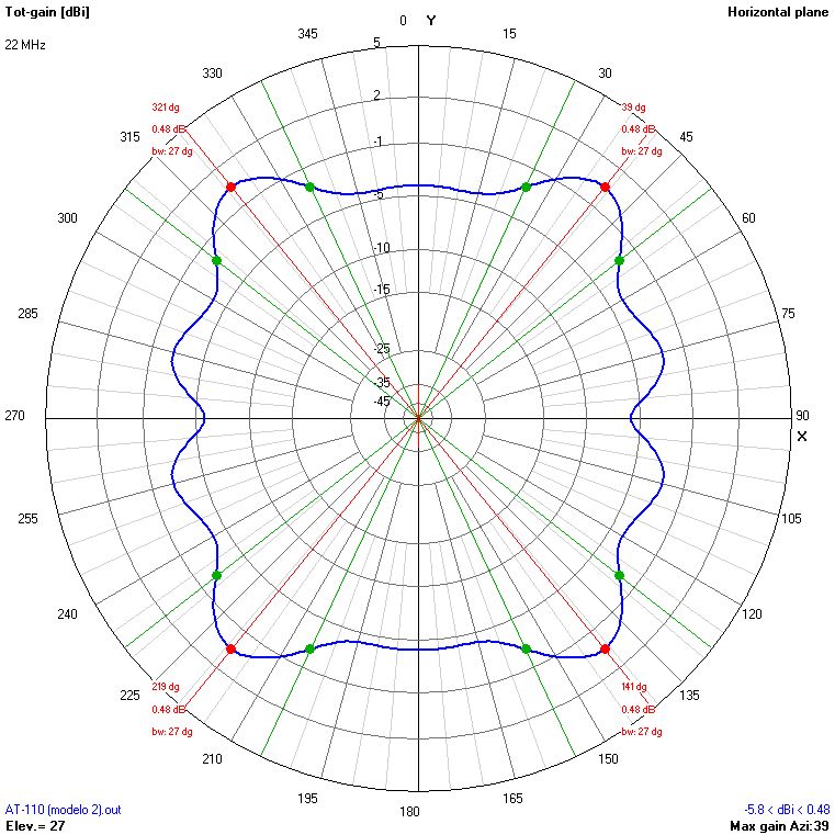 |
 |
 |
 |
 |
 |
 |
 |
| 23 | 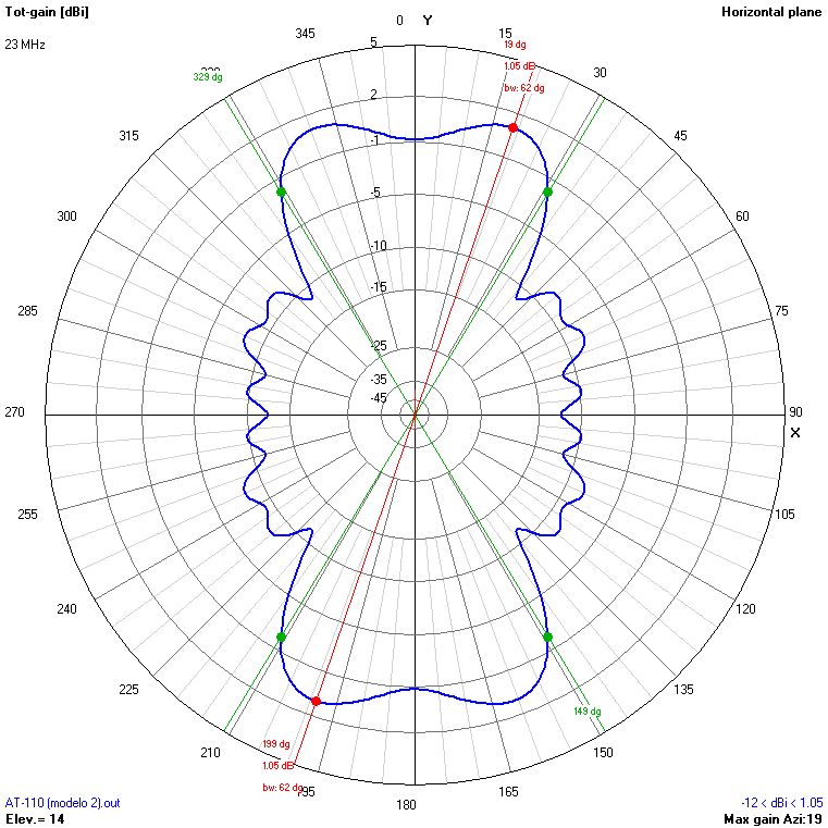 |
 |
 |
 |
 |
 |
 |
 |
| 24 |  |
 |
 |
 |
 |
 |
 |
 |
| 25 | 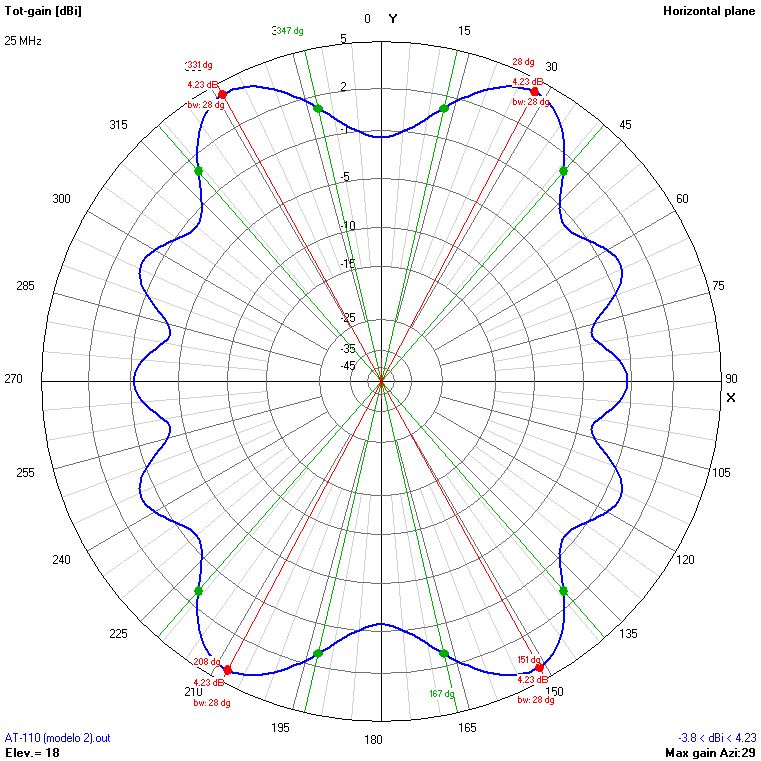 |
 |
 |
 |
 |
 |
 |
 |
| 26 | 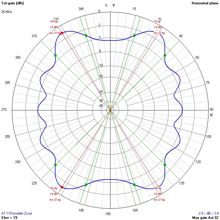 |
 |
 |
 |
 |
 |
 |
 |
| 27 | 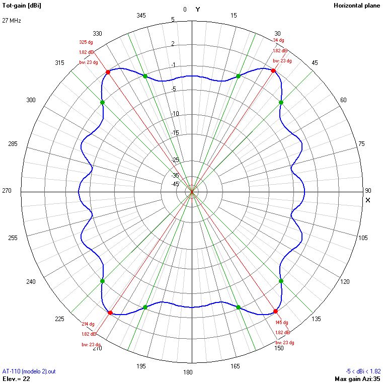 |
 |
 |
 |
 |
 |
 |
 |
| 28 | 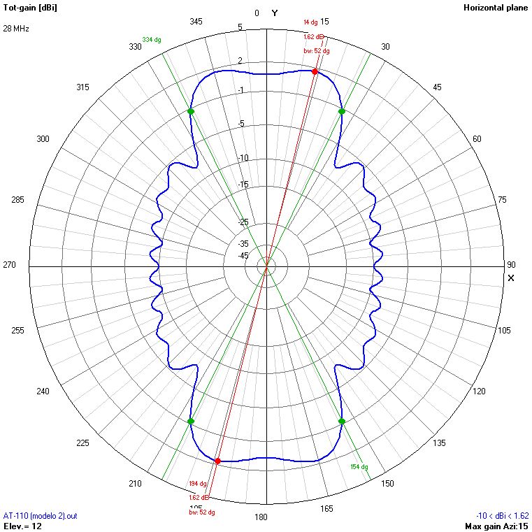 |
 |
 |
 |
 |
 |
 |
 |
| 29 | 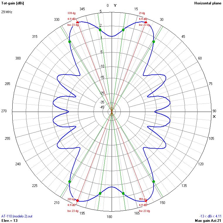 |
 |
 |
 |
 |
 |
 |
 |
| 30 | 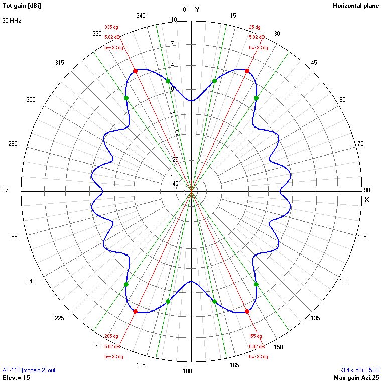 |
 |
 |
 |
 |
 |
 |
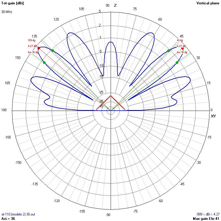 |
Table 8. Radiation patterns of the AT-110A antenna using masts of 9, 12, 15 and 18 metres. Simulation model 2.
Below you will find the plots of maximum gain using masts of 9, 12, 15 and 18 metres. Click on each image to see a larger version.
The figure 12 shows the plot of maximum gain for a height of installation HM = 9 metres.
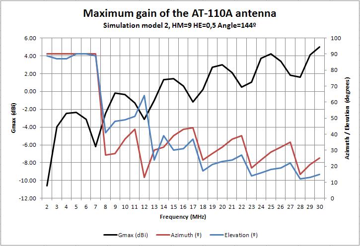
Fig. 12. Maximum gain of the AT-110A antenna with a mast of 9 metres. Simulation model 2.
The figure 13 shows the plot of maximum gain for a height of installation HM = 12 metres.
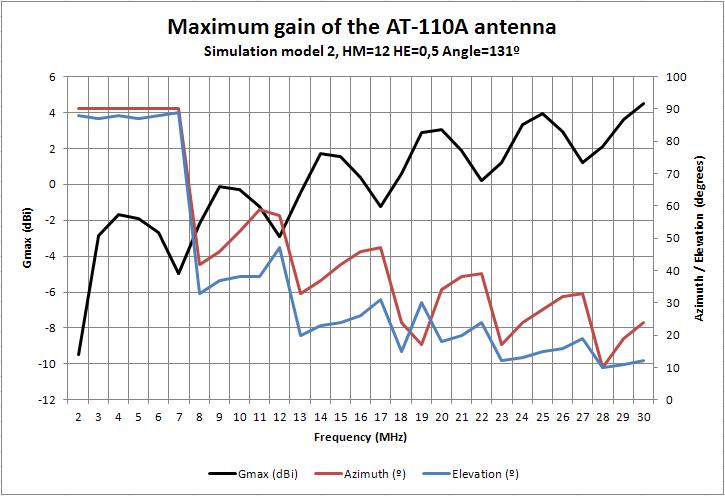
Fig. 13. Maximum gain of the AT-110A antenna with a mast of 12 metres. Simulation model 2.
The figure 14 shows the plot of maximum gain for a height of installation HM = 15 metres.
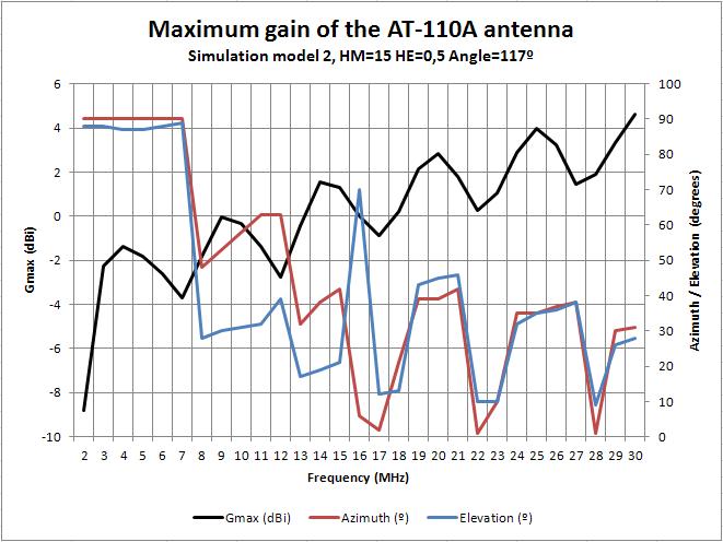
Fig. 14. Maximum gain of the AT-110A antenna with a mast of 15 metres. Simulation model 2.
The figure 15 shows the plot of maximum gain for a height of installation HM = 18 metres.
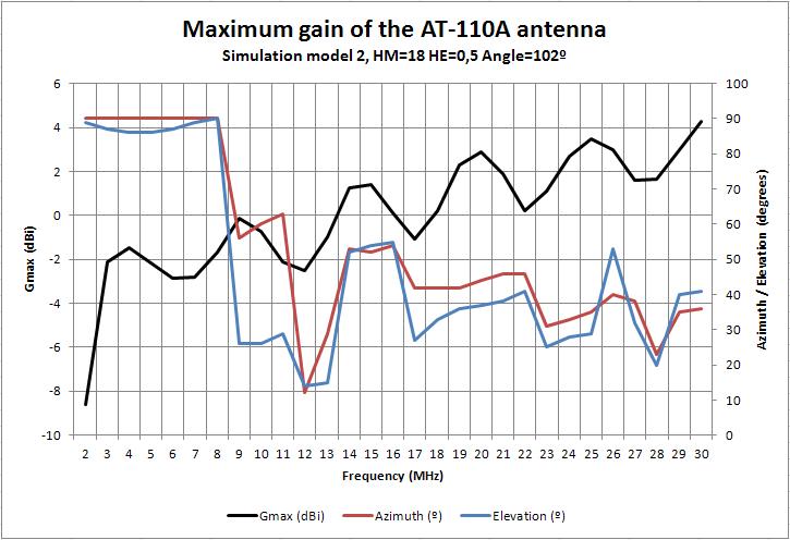
Fig. 15 Maximum gain of the AT-110A antenna with a mast of 18 metres. Simulation model 2.
Finally, the figure 16 shows a comparison of the maximum gain for the four installation configurations analysed.
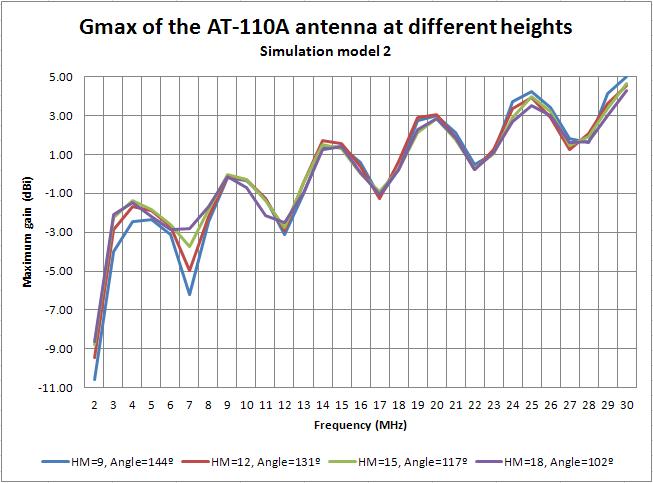
Fig. 16. Comparison of the maximum gain of the AT-110A antenna with different masts. Simulation model 2.
The results will be analysed on the section 7.
7. Results.
In this section I will analyse the results of the simulations made with the two models of the Invelco AT-110A antenna described on the section 2 and using 4NEC2. I have made a total of 408 simulations, counting the convergence and AGT tests and the simulations of SWR and radiation patterns for both models.
The results achieved with both models are quite similar, so the both models can be used to study the antenna’s behaviour under the simulated conditions.
The simulations have been made considering the frequency range from 2 MHz to 30 MHz, installing the antenna in inverted-V configuration over an average terrain and using masts of 9 m, 12 m, 15 m and 18 m.
7.1. Standing wave ratio (SWR).
In both cases (model 1 and model 2), one can see the wideband behaviour of the antenna, with SWR values between 1,01 and 4,76 in the model 1 and between 1,03 and 4,22 in the model 2, all along the whole range 2-30 MHz. Analysing both plots one can conclude the following:
-
The SWR is slightly worse in the lower frequencies.
-
The SWR improves as the height of installation of the antenna increases.
-
The lowest SWR values are seen around 6 MHz, 11 MHz, 16 MHz, 21 MHz and 27 MHz.
-
The highest SWR values are seen around 3 MHz, 8 MHz, 14 MHz, 19 MHz, 24 MHz and 29 MHz.
-
Being a wideband antenna, it is suitable to operate in automatic channel selection modes such as ALE.
Please note that those results may vary as a function of the environment where the antenna is installed (type of ground and nearby obstacles), so in every case it is advisable to use an antenna coupler in order to operate with the antenna. In ideal conditions, it may be enough using the internal coupler of the radio.
7.2. Radiation patterns.
In the simulations performed with both models, one can see similar results relative to the radiation characteristics of the antenna:
-
Regardless the height of installation, the antenna is omnidirectional in frequencies between 2 MHz and about 7 MHz, presenting its maximum of radiation in a direction perpendicular or near perpendicular to the ground. This way, working in those frequencies, the antenna is suitable to establish NVIS links in mobile networks.
-
In frequencies higher than 7 MHz the takeoff angle is lower, between about 10º and 60º of elevation depending on the height of installation of the antenna and the working frequency. The same way, the azimuth angle for the maximum of radiation also depends on the frequency and the height of installation. In previous sections you will find plots to make easier the process of pointing the antenna at the intended station for each case.
-
Being common for HF wideband antennas of these dimensions, the AT-110A has losses in almost half of its working band (lower frequencies), a fact which may be taken into account when assessing the necessary transmission power to establish the links. Anyway, the necessary level of equivalent isotropic radiated power to establish NVIS links is not very high.
-
In the lowest frequencies (up to about 7 MHz), the antenna gain is slightly better when installing the antenna with higher masts. There is no significant improvement in the higher frequencies.